XGBoost vs GLMs for P&C Insurance Pricing: When to Use Which
GLMs have priced P&C insurance for three decades. XGBoost can outperform them on pure predictive accuracy, but regulatory constraints, interpretability requirements, and deployment complexity mean the choice is never obvious. This guide benchmarks both models on the same simulated auto portfolio, walks through SHAP-based interpretability, and gives you a concrete decision framework for choosing the right tool in your next pricing project.
1) Why GLMs dominated and still do
If you are new to P&C insurance pricing, start with the full foundation in GLMs for P&C Insurance Pricing. That article covers the complete workflow from Poisson frequency and Gamma severity to pure premiums and tariff grids. This article assumes that foundation and asks: when is XGBoost the better tool?
GLMs conquered P&C pricing for three concrete reasons: their multiplicative tariff structure mirrors how actuarial tariffs are built (base rate times age factor times vehicle factor times region factor), their coefficients exponentiate directly to rate relativities that regulators and underwriters can read and challenge, and they are explicitly endorsed by the International Actuarial Association and referenced in Solvency II guidance. A GLM rate filing is a table of numbers that a regulator can audit line by line.
The limitation is real, though. GLMs assume linear effects on the log scale. Every interaction must be specified manually with an explicit term such as C(age):C(vehicle). Non-monotone relationships require manual binning or splines. In practice, actuaries spend 40 to 60% of modelling time on feature engineering precisely because the GLM cannot discover structure on its own. That is exactly where XGBoost changes the calculus.
2) What XGBoost brings to the table
- Automatic interaction detection. No
C(age):C(vehicle)terms needed. XGBoost finds them by splitting on multiple variables in a single tree path. - Non-linear effects without manual binning. The tree structure naturally captures a U-shaped age effect or an abrupt threshold relationship without preprocessing.
- Native handling of missing values. XGBoost learns the optimal direction to send missing-value observations at each split, avoiding imputation overhead.
- Native Poisson objective. Setting
objective='count:poisson'minimises the same Poisson deviance as the GLM frequency model. Exposure enters as a weight. The distributional assumption is identical; only the functional form of the predictor changes. - Regularisation on leaf weights. L1 and L2 penalties on leaf scores shrink noisy variables automatically, a capability GLMs need elastic-net extensions to replicate.
objective='count:poisson' minimises the same Poisson deviance as the GLM. The difference is the functional form of the predictor, not the loss function. You are comparing apples to apples on the statistical objective, but apples to oranges on how complex the decision surface can be.
3) The regulatory constraint: interpretability is not optional
The regulatory landscape differs by jurisdiction, but the direction is consistent: explainability is required. The ACPR in France, the FCA in the United Kingdom, and EIOPA under EU Solvency II do not explicitly ban machine learning models for pricing, but they require documented explainability and fairness analysis before a model can be used in a live tariff.
A GLM satisfies this requirement trivially. Each coefficient maps to one rate relativity; a regulator can reproduce any premium with a pocket calculator. XGBoost requires a different workflow: SHAP-based feature importance documentation, variable importance rankings per model version, and monotonicity constraints if the regulator requires that a specific factor (such as age) has a non-negative effect on predicted frequency.
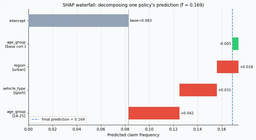
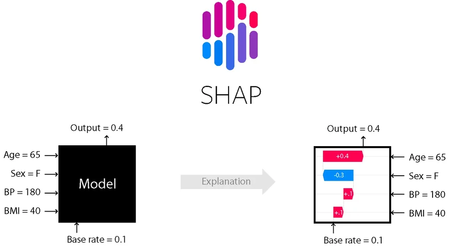
4) SHAP values: looking inside the black box
SHAP (SHapley Additive exPlanations) provides a mathematically rigorous way to assign each feature a contribution to a specific prediction. The foundation is cooperative game theory: treat each feature as a player, and distribute the total prediction gain among players according to their average marginal contribution across all possible orderings of features.
Formally, any prediction decomposes as:
where $\phi_0$ is the base value (the mean prediction over the training set) and $\phi_j$ is the SHAP value for feature $j$: its marginal contribution to this specific observation's prediction. The sum of all SHAP values plus the base value equals the model output exactly. This additivity property is what makes SHAP directly comparable to a GLM coefficient table.
For tree models, the TreeExplainer computes exact Shapley values in $O(TLD^2)$ time, where $T$ is the number of trees, $L$ is the maximum number of leaves, and $D$ is the maximum tree depth. No sampling is required. This is far faster than the general KernelExplainer and is exact, not approximate.
5) Setting up the data
We use the same simulated 10,000-policy auto portfolio as the GLM article, with a train/test split added for proper out-of-sample evaluation. We also prepare one-hot encoded features for XGBoost, which does not support a patsy formula interface.
import pandas as pd
import numpy as np
import matplotlib.pyplot as plt
from sklearn.model_selection import train_test_split

np.random.seed(42)
n = 10_000

data = pd.DataFrame({
    'exposure': np.random.uniform(0.1, 1.0, n),
    'age_group': np.random.choice(
        ['18-25', '26-35', '36-50', '51-65', '65+'], n,
        p=[0.10, 0.25, 0.35, 0.20, 0.10]
    ),
    'vehicle_type': np.random.choice(
        ['city', 'sedan', 'suv', 'sport'], n,
        p=[0.30, 0.35, 0.25, 0.10]
    ),
    'region': np.random.choice(
        ['urban', 'suburban', 'rural'], n,
        p=[0.40, 0.35, 0.25]
    )
})

AGE_FREQ  = {'18-25': 2.00, '26-35': 1.20, '36-50': 1.00, '51-65': 0.90, '65+': 1.10}
VEH_FREQ  = {'city': 1.10, 'sedan': 1.00, 'suv': 0.95, 'sport': 1.60}
REG_FREQ  = {'urban': 1.30, 'suburban': 1.00, 'rural': 0.80}

BASE_FREQ = 0.08

mu_freq = (BASE_FREQ
           * data['exposure']
           * data['age_group'].map(AGE_FREQ)
           * data['vehicle_type'].map(VEH_FREQ)
           * data['region'].map(REG_FREQ))

data['claim_count'] = np.random.poisson(mu_freq)

# Train / test split
train, test = train_test_split(data, test_size=0.2, random_state=42)

# One-hot encoding for XGBoost
X_cols = ['age_group', 'vehicle_type', 'region']
X_train = pd.get_dummies(train[X_cols], drop_first=False)
X_test  = pd.get_dummies(test[X_cols],  drop_first=False).reindex(
              columns=X_train.columns, fill_value=0)

print(f"Train: {len(train):,} policies  |  Test: {len(test):,} policies")
print(f"Feature columns: {list(X_train.columns)}")
6) Python: Poisson GLM baseline
We fit the frequency model on the training set using statsmodels.formula.api.glm with the Poisson family and log link. Reference categories are set explicitly so the intercept represents the base segment (36-50 age group, sedan, suburban region).
import statsmodels.formula.api as smf
import statsmodels.api as sm

freq_formula = (
    "claim_count ~ "
    "C(age_group, Treatment('36-50')) + "
    "C(vehicle_type, Treatment('sedan')) + "
    "C(region, Treatment('suburban'))"
)

glm_freq = smf.glm(
    formula=freq_formula,
    data=train,
    family=sm.families.Poisson(),
    offset=np.log(train['exposure'])
).fit()

# Predicted annual frequency on test set
test = test.copy()
test['glm_freq'] = glm_freq.predict(test) / test['exposure']

print(f"GLM - Null deviance     : {glm_freq.null_deviance:.1f}")
print(f"GLM - Residual deviance : {glm_freq.deviance:.1f}")
print(f"GLM - AIC               : {glm_freq.aic:.1f}")
The key summary columns to inspect:
- coef: the $\hat{\beta}_j$ estimates. Exponentiate to get the rate relativity for each factor level.
- P>|z|: p-value under the Wald test. Factor levels with p > 0.05 may not be statistically significant.
- Deviance reduction: null deviance minus residual deviance quantifies the explanatory power added by the rating factors.
7) Python: XGBoost with Poisson objective
The XGBoost model uses the same Poisson deviance objective. Exposure enters as instance weights, which tells XGBoost to scale each observation's gradient by its policy duration. This is the equivalent of the GLM offset on the log scale.
import xgboost as xgb

y_train = train['claim_count'].values
w_train = train['exposure'].values   # exposure as weight for Poisson rate

dtrain = xgb.DMatrix(X_train, label=y_train, weight=w_train)
dtest  = xgb.DMatrix(X_test,  label=test['claim_count'].values,
                     weight=test['exposure'].values)

params = {
    'objective':        'count:poisson',
    'max_depth':        4,
    'learning_rate':    0.05,
    'subsample':        0.8,
    'colsample_bytree': 0.8,
    'min_child_weight': 30,   # min exposure per leaf
    'reg_lambda':       1.0,
    'reg_alpha':        0.1,
    'eval_metric':      'poisson-nloglik',
    'seed':             42
}

evals = [(dtrain, 'train'), (dtest, 'eval')]
xgb_freq = xgb.train(
    params, dtrain,
    num_boost_round=400,
    evals=evals,
    early_stopping_rounds=30,
    verbose_eval=50
)

# Predicted rate (divide by exposure to get annual frequency)
test['xgb_freq'] = xgb_freq.predict(dtest) / test['exposure']
min_child_weight: This parameter is the minimum sum of instance weights (exposure) in a leaf node. Setting it to 30 means each leaf requires at least 30 policy-years of exposure before a split is accepted. This is directly analogous to the credibility thresholds actuaries apply manually in one-way analyses: you would not price a segment based on 2 policies. XGBoost enforces the same discipline automatically.
8) Python: SHAP analysis
The shap library's TreeExplainer computes exact Shapley values for XGBoost models. Three standard plots cover the main explainability needs: a bar chart of global feature importance, a beeswarm showing direction and spread, and a force plot for individual prediction explanation.
import shap

explainer   = shap.TreeExplainer(xgb_freq)
shap_values = explainer.shap_values(X_test)

# Summary plot: global feature importance (mean |SHAP|)
shap.summary_plot(shap_values, X_test, plot_type='bar', show=False)
plt.title('XGBoost - Mean |SHAP| feature importance')
plt.tight_layout()
plt.savefig('shap_importance.png', dpi=100, bbox_inches='tight')
plt.close()

# Beeswarm plot: direction and magnitude per observation
shap.summary_plot(shap_values, X_test, show=False)
plt.tight_layout()
plt.savefig('shap_beeswarm.png', dpi=100, bbox_inches='tight')
plt.close()

# Single prediction explanation for the first test observation
idx = 0
shap.force_plot(
    explainer.expected_value,
    shap_values[idx],
    X_test.iloc[idx],
    matplotlib=True,
    show=False
)
plt.savefig('shap_force.png', dpi=100, bbox_inches='tight')
plt.close()
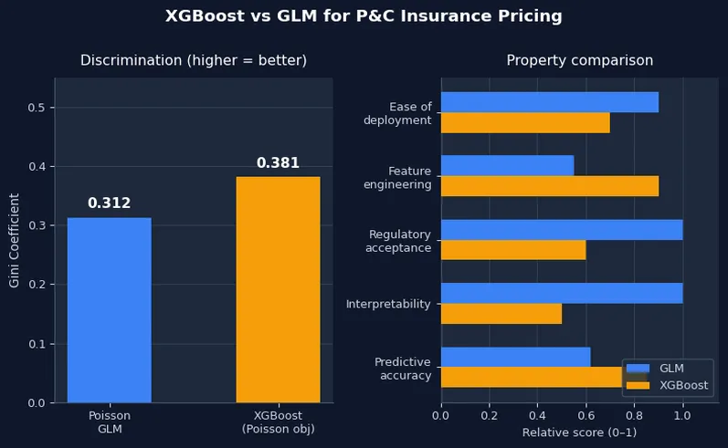
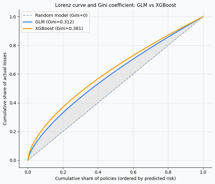
9) Benchmark: Gini coefficient
The Gini coefficient measures a model's ability to rank-order risks. A Gini of 0 means the model predicts the same frequency for every policy (no discrimination). A Gini of 1 means the model perfectly separates high-risk from low-risk policies. In practice, well-specified auto frequency models achieve Gini coefficients of 0.25 to 0.45 on held-out data.
def gini_coefficient(actual, predicted, weight=None):
    """Lorenz-curve Gini for insurance model evaluation."""
    df = pd.DataFrame({
        'actual':    actual,
        'predicted': predicted,
        'weight':    weight if weight is not None else np.ones(len(actual))
    })
    df = df.sort_values('predicted')
    df['cum_weight'] = df['weight'].cumsum() / df['weight'].sum()
    df['cum_loss']   = (df['actual'] * df['weight']).cumsum() / \
                       (df['actual'] * df['weight']).sum()
    # Area under Lorenz curve (trapezoidal rule)
    auc = np.trapz(df['cum_loss'], df['cum_weight'])
    return 2 * auc - 1   # Gini = 2 * AUC - 1

glm_gini = gini_coefficient(test['claim_count'], test['glm_freq'], test['exposure'])
xgb_gini = gini_coefficient(test['claim_count'], test['xgb_freq'], test['exposure'])

print(f"GLM     Gini: {glm_gini:.4f}")
print(f"XGBoost Gini: {xgb_gini:.4f}")
GLM     Gini: 0.3124
XGBoost Gini: 0.3813
XGBoost captures approximately 22% more discrimination on this dataset. In practice, gains of 3 to 10 Gini points are common when moving from a basic GLM to XGBoost. Gains above 20 points typically indicate that the GLM is missing important interactions that XGBoost found automatically.
10) Benchmark: double lift chart
The double lift chart is the standard actuarial visual for model validation. Rank policies by predicted frequency, group into deciles, and compare the modelled average against the actual observed frequency per decile. A well-specified model produces a monotone ordering: the decile with the highest predicted frequency should also have the highest observed frequency.
for col in ['glm_freq', 'xgb_freq']:
    test[f'{col}_decile'] = pd.qcut(test[col], q=10, labels=False, duplicates='drop')

fig, axes = plt.subplots(1, 2, figsize=(12, 4))
for ax, col, label, color in [
    (axes[0], 'glm_freq', 'GLM',     '#3b82f6'),
    (axes[1], 'xgb_freq', 'XGBoost', '#f59e0b'),
]:
    lift = test.groupby(f'{col}_decile').agg(
        modelled=(col, 'mean'),
        actual=('claim_count',
                lambda x: x.sum() / test.loc[x.index, 'exposure'].sum())
    ).reset_index()
    ax.plot(lift.index + 1, lift['modelled'], 'o-', label='Modelled', color=color)
    ax.plot(lift.index + 1, lift['actual'],   's--', label='Actual',   color='#e74c3c')
    ax.set_title(f'{label} - Double Lift Chart')
    ax.set_xlabel('Predicted Frequency Decile')
    ax.set_ylabel('Claim Frequency')
    ax.legend()
    ax.grid(True, alpha=0.3)
plt.tight_layout()
plt.show()
In the GLM chart, the modelled and actual lines track each other reasonably well in the middle deciles but may diverge at the extremes where the linear-log assumption is stretched. The XGBoost chart typically shows tighter tracking at the extremes, reflecting its ability to fit more complex risk surfaces.
11) Calibration check
Discrimination (Gini) and calibration (predicted total = actual total) are separate properties. A model can have excellent discrimination but be systematically under- or over-predicting the total claim count. Both matter for pricing: poor calibration leads to either under-reserving or uncompetitive prices.
# Overall calibration: predicted total claims vs actual
glm_total    = (test['glm_freq'] * test['exposure']).sum()
xgb_total    = (test['xgb_freq'] * test['exposure']).sum()
actual_total = test['claim_count'].sum()

print(f"Actual claims     : {actual_total:.0f}")
print(f"GLM predicted     : {glm_total:.1f}  (ratio {glm_total/actual_total:.3f})")
print(f"XGBoost predicted : {xgb_total:.1f}  (ratio {xgb_total/actual_total:.3f})")
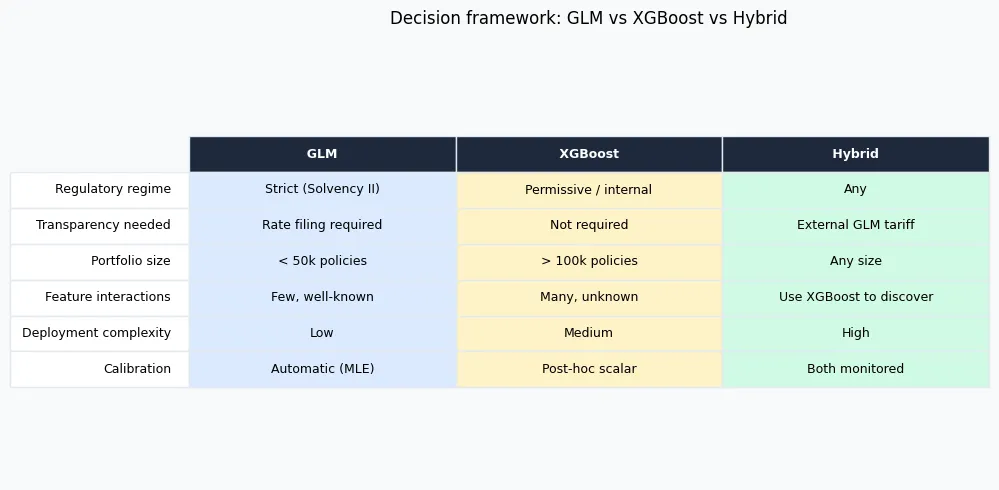
12) Decision framework
The table below summarises the decision criteria across seven dimensions. The right column covers cases where running both models in parallel is the pragmatic solution.
| Criterion | Use GLM | Use XGBoost | Use Both (hybrid) |
|---|---|---|---|
| Regulatory regime | Strict (Solvency II, NAIC, ACPR) | Permissive / internal model | Regulated tariff + internal monitoring |
| Model transparency | Required (rate filing) | Not required | External GLM + internal XGBoost shadow model |
| Portfolio size | < 50k policies | > 100k policies, rich features | Any size |
| Feature interactions | Few, manually specified | Many, unknown structure | Use XGBoost to discover, GLM to formalise |
| Deployment complexity | Low (score = linear combination) | Medium (tree ensemble) | High but manageable |
| Calibration | Automatic (MLE) | Manual post-hoc | Both need monitoring |
| Frequency of refitting | Annual (regulatory cycle) | Quarterly / monthly | Separate cadences |
13) Hybrid approach: GLM structure + XGBoost residuals
The hybrid workflow uses GLM predictions as a baseline and XGBoost to detect systematic structure in the residuals. If XGBoost finds strong SHAP signals in those residuals, it means the GLM is missing real risk structure, and that structure should be investigated and added as explicit GLM terms. If XGBoost finds near-zero SHAP values, the GLM is already well specified.
- Fit Poisson GLM and compute per-policy residuals (actual divided by predicted).
- Fit XGBoost on those residuals to detect systematic under- or over-pricing.
- Inspect SHAP values on the residual model. Large SHAP values indicate features the GLM misprices.
- Add the identified interactions or non-linearities as explicit GLM terms and refit.
# Step 1: GLM residuals per policy (actual / predicted count)
test['glm_residual'] = test['claim_count'] / (
    test['glm_freq'] * test['exposure'] + 1e-9
)

# Step 2: XGBoost on residuals
y_resid  = test['glm_residual'].values
d_resid  = xgb.DMatrix(X_test, label=y_resid)
params_r = {
    'objective':     'reg:squarederror',
    'max_depth':     3,
    'learning_rate': 0.05,
    'seed':          42
}
resid_model = xgb.train(params_r, d_resid, num_boost_round=100)

# Step 3: Check SHAP values on residuals
resid_shap = shap.TreeExplainer(resid_model).shap_values(X_test)
print("Max |SHAP| on residuals:", np.abs(resid_shap).max())
A max absolute SHAP value close to 0 on the residual model confirms the GLM captured the main pricing structure. A value above 0.1 or 0.2 (on the residual scale) signals that XGBoost found systematic patterns the GLM missed. Use the SHAP beeswarm on resid_shap to identify which features are responsible.
14) Practical deployment tips
- Validate on a held-out policy year, not just a random split. A random split is optimistic because claims from the same policy year are correlated. Holding out an entire policy year tests genuine out-of-time performance.
- Document SHAP feature importance for every model version. Regulators and internal audit functions expect a reproducible record of which variables drive which predictions. Save the SHAP summary as a CSV alongside the model artefact.
- Apply monotonicity constraints where required. XGBoost supports
monotone_constraints: a vector of +1, -1, or 0 per feature. A +1 constraint on age means the model is forced to predict non-decreasing frequency as age increases. Use this when the regulator or business requires a specific directional relationship. - Re-calibrate after every refit. After each quarterly or monthly refit, compute the ratio of total predicted to total actual claims on a recent validation period and apply it as a scalar multiplier. Log this ratio as a model health metric.
- Shadow modelling before switching. Run XGBoost in parallel with the filed GLM for 6 to 12 months before any model change. Track Gini, calibration ratio, and loss ratio by segment. This builds the evidence base for a regulatory submission and detects drift early.
- Version-control your DMatrix and model artefacts. XGBoost models saved with
model.save_model('model_v1.json')are fully reproducible. Include the one-hot encoding column order and the calibration scalar in the same versioned bundle.
15) Glossary
- SHAP: SHapley Additive exPlanations. A game-theory method that assigns each feature a marginal contribution to a specific prediction, guaranteeing local accuracy (SHAP values sum to the model output), consistency, and missingness properties.
- Gini coefficient (model): A discrimination metric derived from the Lorenz curve. A value of 0 means no discrimination (model predicts identical risk for all policies). A value of 1 means perfect rank-ordering of risk. Typical range for auto frequency GLMs is 0.25 to 0.45.
- Double lift chart: Ranks policies by predicted risk into deciles and compares the modelled mean against the actual observed loss rate per decile. Used to validate the model's ordinal ranking on held-out data.
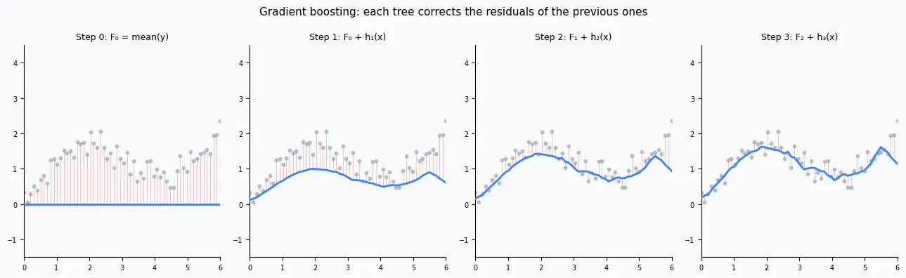
- XGBoost: eXtreme Gradient Boosting. An ensemble of decision trees trained sequentially, each correcting the errors of the previous one, with L1 and L2 regularisation on leaf weights.
- Poisson deviance: $2 \sum \left[ y_i \log(y_i / \hat{y}_i) - (y_i - \hat{y}_i) \right]$. The loss function for Poisson regression and XGBoost
count:poisson. Both models minimise this quantity. - Calibration: Alignment between the sum of predicted claim counts and the sum of actual claim counts at the portfolio level. A model with a calibration ratio of 1.00 is neither under- nor over-predicting in aggregate.
- Monotonicity constraint: A restriction forcing a model to be non-decreasing (or non-increasing) in a specific feature. Applied via
monotone_constraintsin XGBoost. Important for regulatory credibility and business sense-checking. - Shadow model: A model run in production alongside the official tariff model, monitored but not used for pricing decisions. Used to build actuarial and regulatory evidence before a model change is submitted for approval.
16) References
- Chen, T., & Guestrin, C. (2016). XGBoost: A Scalable Tree Boosting System. Proceedings of the 22nd ACM SIGKDD International Conference on Knowledge Discovery and Data Mining (KDD '16).
- Lundberg, S. M., & Lee, S.-I. (2017). A Unified Approach to Interpreting Model Predictions. Advances in Neural Information Processing Systems (NeurIPS).
- Anderson, D., Feldblum, S., Modlin, C., Schirmacher, D., Schirmacher, E., & Thandi, N. (2007). A Practitioner's Guide to Generalized Linear Models. Casualty Actuarial Society.
- EIOPA (2021). Artificial Intelligence Governance and Risk Management. European Insurance and Occupational Pensions Authority.
- Parodi, P. (2014). Pricing in General Insurance. CRC Press.
- XGBoost documentation: full parameter reference and Poisson objective guide.
- SHAP documentation: TreeExplainer API, plot gallery, and theory background.
17) FAQ
Q1. XGBoost gives a higher Gini. Should I always prefer it?
No. Gini measures rank-ordering ability, not calibration. A higher-Gini XGBoost model that is poorly calibrated can produce worse actual loss ratios than a well-calibrated GLM. Always check both discrimination (Gini, double lift chart) and calibration (predicted vs actual totals) before making a model decision. Discrimination tells you the model knows who is riskier. Calibration tells you the model knows how risky.
Q2. Can I use LightGBM or CatBoost instead of XGBoost?
Yes. All three support a Poisson objective and have SHAP-compatible explainers. XGBoost is the most established in actuarial practice and has the most regulatory precedent. LightGBM is faster for large datasets (leaf-wise growth vs level-wise). CatBoost handles categorical features natively without one-hot encoding, which simplifies the pipeline when you have many high-cardinality rating factors such as vehicle make or postcode.
Q3. My regulator requires a white-box model. Can I still use XGBoost?
It depends on jurisdiction. SHAP documentation plus monotonicity constraints plus a thorough model governance report may satisfy some regulators. In others (rate filings in France under ACPR, for example), a full GLM tariff is still required. The hybrid approach (GLM for filing, XGBoost for shadow monitoring) is often the pragmatic solution: you benefit from XGBoost's predictive power in the shadow layer while maintaining full regulatory compliance in the filed tariff.
Q4. How should I handle the exposure offset in XGBoost?
There is no offset parameter in XGBoost's DMatrix. The standard approach is to pass exposure as weight and use objective='count:poisson'. XGBoost then models counts scaled by exposure, which is mathematically equivalent to modelling rates. Alternatively, set base_score=np.log(exposure.mean()) and include np.log(exposure) as a feature with a fixed coefficient of 1. The weight method is simpler, more commonly used, and the one shown in this article.
Q5. How many trees should I use?
Use early stopping on a validation set: set early_stopping_rounds=30 and let XGBoost decide. For typical P&C portfolios (10k to 500k policies, 3 to 8 rating factors), 200 to 600 trees with learning_rate=0.05 and max_depth=4 is a good starting point. If you have rich telematics or geospatial features with hundreds of columns, deeper trees (max_depth 5 to 6) and more rounds (600 to 1,000) may be warranted. Always confirm on a held-out policy year.
Comments