GLMs for P&C Insurance Pricing: A Practical Guide with Python
Generalized Linear Models have been the industry backbone of P&C insurance pricing for over thirty years. This guide walks you through the complete pricing workflow: why the multiplicative GLM structure fits the problem, how to model claim frequency with Poisson regression and claim severity with Gamma regression, and how to combine both into a pure premium that drives your tariff. All theory is backed by a full Python implementation you can run on simulated auto insurance data.
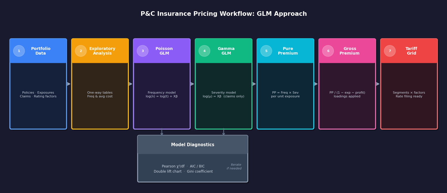
The end-to-end pricing workflow. Each step is covered in full below.
1) What is P&C insurance?
P&C stands for Property & Casualty — the broad family of insurance products that protect against physical damage to assets and liability arising from accidents. It is also called non-life insurance or general insurance in many markets. If you own a car, a home, or run a business, you are almost certainly a P&C policyholder.
- Personal auto: covers collisions, theft, and third-party liability for private drivers.
- Homeowners / property: covers fire, flood, burglary, and structural damage to buildings and contents.
- Commercial liability: protects businesses against claims made by third parties for bodily injury or property damage.
- Workers' compensation: covers employees injured on the job.
- Marine & transport: covers cargo, vessels, and freight in transit.
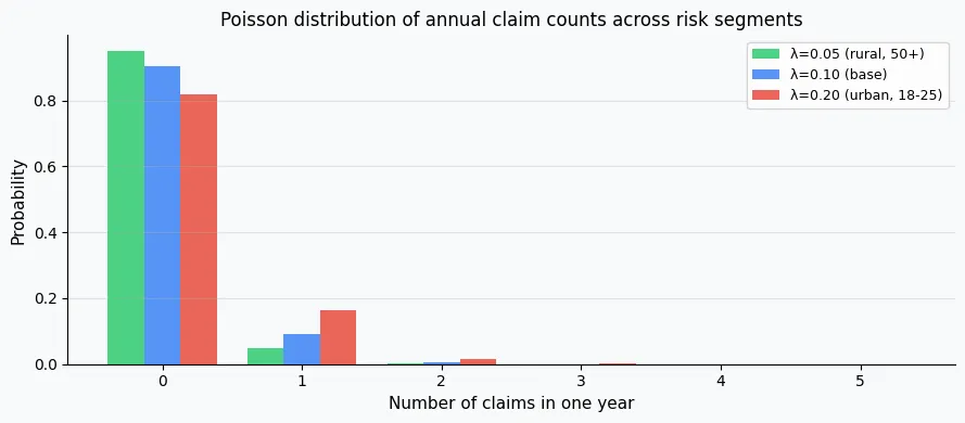
Unlike life insurance — where the insured event (death) is certain, just unknown in timing — P&C events are random in both occurrence and severity. Most policyholders will never claim in a given year. A small minority will claim once. An even smaller minority will have several claims. This randomness is precisely what makes statistical modelling so valuable.
How does insurance work financially?
The insurance company collects a premium from each policyholder upfront, then pays claims (losses) when covered events occur. The basic financial equation is:
For the insurer to remain solvent and competitive:
- Too low a premium: the insurer collects less than it pays out — losses erode capital, eventually leading to insolvency.
- Too high a premium: policyholders switch to cheaper competitors. Market share collapses.
The pricing actuary's job is to find the technically correct premium for each policyholder: one that reflects their individual risk profile, is sustainable for the insurer, and is competitive in the market.
Key concepts you need to know
| Term | Definition | Example |
|---|---|---|
| Policy | The contract between the insurer and the insured. | 12-month auto insurance contract for a specific vehicle. |
| Premium | The amount the policyholder pays for coverage. | £850/year for a 30-year-old driving a sedan. |
| Claim | A request for payment after a covered loss event. | Filing for £3,200 after a rear-end collision. |
| Exposure | The unit of risk — typically policy-years in force. | A 6-month policy contributes 0.5 policy-years of exposure. |
| Loss ratio | Claims paid ÷ premiums earned. Target is typically 60–75%. | Loss ratio of 0.68 means £68 in claims per £100 of premium. |
| Rating factor | A policyholder characteristic used to differentiate risk. | Driver age, vehicle type, region, annual mileage. |
| Pure premium | Expected loss cost per unit of exposure, before loadings. | A segment with pure premium £210/year needs at least £210 in premium before expenses and profit. |
Why can't the insurer charge everyone the same price?
Imagine a portfolio of 1,000 drivers all paying a flat £500 premium. The insurer collects £500,000. In reality, 50 drivers have a claim averaging £8,000 each — total losses of £400,000. The portfolio breaks even on paper.
But now suppose the 50 claimants are all young urban drivers with sports cars. The other 950 drivers — mostly older, rural, driving modest cars — are subsidising a group they have nothing in common with. If a competitor enters the market and offers low-risk drivers a £300 premium (accurate to their risk), the insurer loses its best risks, retains only the bad ones, and faces losses. This is called adverse selection.
The solution is risk segmentation: split the portfolio into groups with similar risk profiles and charge each group a price that reflects its expected cost. That is exactly what GLMs do — and it is where the rest of this article begins.
2) Why GLMs dominate P&C pricing
Before GLMs became standard in the 1990s, actuaries built tariffs using one-way analyses: they would look at each rating factor (age, vehicle type, region) in isolation and compute observed loss ratios. The approach ignored interactions and correlations between factors, leading to biased prices.
GLMs solve this by adjusting all factors simultaneously. The regression controls for confounding: if young drivers also happen to drive sports cars, GLM separates the age effect from the vehicle effect. The key properties that make GLMs the right tool for pricing:
- Multiplicative structure. Rate relativities multiply, which is how tariffs are built: base rate × age factor × vehicle factor × region factor.
- Correct distributional assumption. Claim counts are non-negative integers (Poisson). Claim amounts are positive and right-skewed (Gamma). Ordinary regression assumes Gaussian errors: wrong for both.
- Exposure offset. Policies have different durations. A policy in force for 6 months contributes half the exposure of a full-year policy. GLMs handle this naturally via an offset term.
- Interpretable coefficients. Each coefficient $\hat{\beta}_j$ exponentiates to a rate relativity: the multiplicative premium adjustment for that factor level relative to the base.
- Regulatory acceptance. GLMs are endorsed by the International Actuarial Association and referenced in Solvency II guidance.
3) GLM structure: the three components
A GLM generalises ordinary linear regression along three axes:
1. Random component: the distribution of the response $Y$. Must be from the exponential family: Poisson, Gamma, Gaussian, Binomial, Tweedie, etc.
2. Systematic component: the linear predictor $\eta = \mathbf{X}\boldsymbol{\beta}$, a weighted sum of the explanatory variables.
3. Link function $g(\cdot)$: connects the expected response to the linear predictor: $g(\mu) = \eta$.
For a single observation $i$, the model reads:
Parameters are estimated by Maximum Likelihood Estimation (MLE), not least squares. For the Poisson and Gamma families, the MLE has a closed-form score equation and is solved iteratively using Iteratively Reweighted Least Squares (IRLS).
4) The exponential family: why it matters for pricing
A GLM's random component must belong to the exponential family — a large class of distributions that share a common mathematical form. Understanding this form explains WHY Poisson fits claim counts and WHY Gamma fits claim costs.
The canonical exponential family density is:
Each term plays a specific role:
- $\theta$: natural (canonical) parameter, linked to the mean
- $b(\theta)$: cumulant function; its derivatives give the mean and variance: $\mu = b'(\theta)$, $\text{Var}(Y) = a(\phi)\,b''(\theta)$
- $a(\phi)$: dispersion function
- $c(y,\phi)$: normalising term (does not affect inference on $\theta$)
The table below shows how the key distributions used in P&C pricing fit into this framework:
| Distribution | Support | $b(\theta)$ | Mean $\mu$ | Variance | Insurance use |
|---|---|---|---|---|---|
| Poisson | $\{0,1,2,...\}$ | $e^\theta$ | $e^\theta$ | $\mu$ | Claim counts |
| Gamma | $(0, \infty)$ | $-\ln(-\theta)$ | $-1/\theta$ | $\phi\mu^2$ | Claim amounts |
| Gaussian | $(-\infty,\infty)$ | $\theta^2/2$ | $\theta$ | $\phi$ | Not used (negative values possible) |
| Tweedie | $[0,\infty)$ | power-law | power of $\mu$ | $\phi\mu^p$ | Aggregate losses |
GLM parameters are estimated by Maximum Likelihood. The log-likelihood for the exponential family is:
Setting $\partial\ell/\partial\boldsymbol{\beta} = 0$ yields the score equations, solved iteratively by IRLS (Iteratively Reweighted Least Squares). In practice, statsmodels handles this automatically.
5) Claim frequency: Poisson regression
The frequency model predicts the expected number of claims a policy will generate over its exposure period. The natural distribution for count data is the Poisson:
With the canonical log link and an exposure offset $t_i$ (years in force):
The offset $\log(t_i)$ ensures we model the rate of claims per unit time, not just the raw count. This is critical: a policy active for 3 months is not directly comparable to one active for 12 months without adjusting for exposure.
The model for claim frequency per unit exposure is:
6) Claim severity: Gamma regression
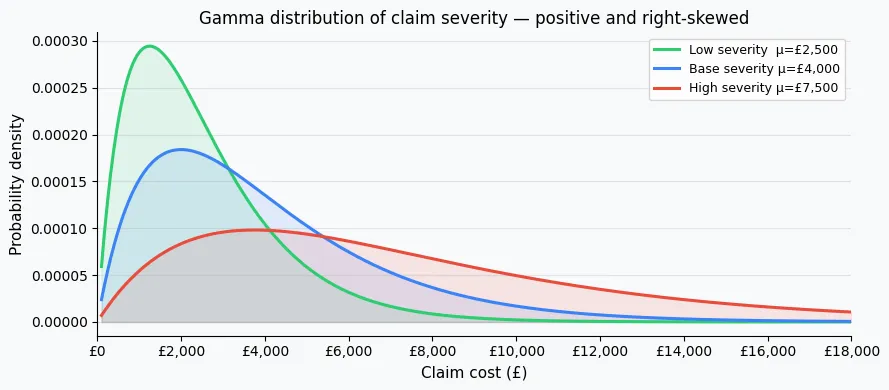
The severity model predicts the average cost per claim, fitted on the sub-portfolio of policies that actually had at least one claim. Claim amounts are strictly positive and right-skewed: well described by the Gamma distribution:
The variance is proportional to $\mu^2$, meaning the coefficient of variation $\text{CV} = \sqrt{\phi}$ is constant across all segments. This is typically a better fit than assuming constant variance (Gaussian) or variance proportional to $\mu$ (Poisson).
With the log link:
claim_count > 0). Including zero-claim policies would conflate frequency and severity effects.
7) Pure premium = Frequency × Severity
The pure premium (also called the burning cost) is the expected loss per unit of exposure. It decomposes into:
Because both models use a log link, the pure premium is also multiplicative:
The gross premium is then the pure premium loaded for expenses, profit margin, and reinsurance cost:
8) Why the log link matters
The choice of link function shapes the interpretation. With the log link, each coefficient $\hat{\beta}_j$ exponentiates to a rate relativity:
The multiplicative structure means relativities chain correctly:
This is exactly how manual tariff tables work, but now the numbers come from a statistically rigorous MLE estimation rather than one-way averages.
9) Setting up your data
A typical P&C pricing dataset has one row per policy (or per policy-year). The minimum required columns are:
- exposure: years in force (e.g., 0.5 for a 6-month policy)
- claim_count: total number of claims reported during the period
- claim_amount: total incurred loss amount for the period
- Rating factors: age group, vehicle type, region, bonus-malus level, etc.
We simulate a 10,000-policy auto portfolio to illustrate the full workflow:
import pandas as pd
import numpy as np
import statsmodels.api as sm
import statsmodels.formula.api as smf
import matplotlib.pyplot as plt
np.random.seed(42)
n = 10_000
data = pd.DataFrame({
'exposure': np.random.uniform(0.1, 1.0, n),
'age_group': np.random.choice(
['18-25', '26-35', '36-50', '51-65', '65+'], n,
p=[0.10, 0.25, 0.35, 0.20, 0.10]
),
'vehicle_type': np.random.choice(
['city', 'sedan', 'suv', 'sport'], n,
p=[0.30, 0.35, 0.25, 0.10]
),
'region': np.random.choice(
['urban', 'suburban', 'rural'], n,
p=[0.40, 0.35, 0.25]
)
})
# True multiplicative relativities (ground truth for validation)
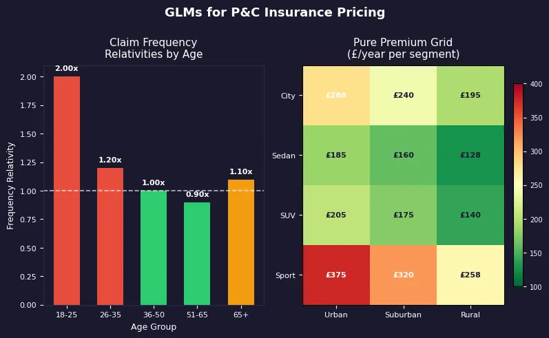
AGE_FREQ = {'18-25': 2.00, '26-35': 1.20, '36-50': 1.00, '51-65': 0.90, '65+': 1.10}
VEH_FREQ = {'city': 1.10, 'sedan': 1.00, 'suv': 0.95, 'sport': 1.60}
REG_FREQ = {'urban': 1.30, 'suburban': 1.00, 'rural': 0.80}
AGE_SEV = {'18-25': 1.30, '26-35': 1.10, '36-50': 1.00, '51-65': 0.95, '65+': 1.05}
VEH_SEV = {'city': 0.90, 'sedan': 1.00, 'suv': 1.20, 'sport': 1.50}
REG_SEV = {'urban': 1.10, 'suburban': 1.00, 'rural': 0.90}
BASE_FREQ = 0.08 # 8% claim rate per year
BASE_SEV = 2_500 # base claim cost (£)
mu_freq = (BASE_FREQ
* data['exposure']
* data['age_group'].map(AGE_FREQ)
* data['vehicle_type'].map(VEH_FREQ)
* data['region'].map(REG_FREQ))
mu_sev = (BASE_SEV
* data['age_group'].map(AGE_SEV)
* data['vehicle_type'].map(VEH_SEV)
* data['region'].map(REG_SEV))
data['claim_count'] = np.random.poisson(mu_freq)
mask = data['claim_count'] > 0
data['claim_amount'] = 0.0
data.loc[mask, 'claim_amount'] = np.random.gamma(
shape=2.0, scale=mu_sev[mask] / 2.0
)
print(f"Policies : {n:,}")
print(f"With claims : {mask.sum():,} ({mask.mean()*100:.1f}%)")
print(f"Avg claim count : {data['claim_count'].mean():.4f}")
print(f"Avg severity : £{data.loc[mask, 'claim_amount'].mean():,.0f}")
10) Python: Poisson frequency model
We fit the frequency model using statsmodels.formula.api.glm with a Poisson family and log link. The reference category for each factor is set explicitly with Treatment() so the intercept represents the base segment.
# ── FREQUENCY MODEL ──────────────────────────────────────────────────────
freq_formula = (
    "claim_count ~ "
    "C(age_group, Treatment('36-50')) + "
    "C(vehicle_type, Treatment('sedan')) + "
    "C(region, Treatment('suburban'))"
)

freq_model = smf.glm(
    formula=freq_formula,
    data=data,
    family=sm.families.Poisson(),
    offset=np.log(data['exposure'])
).fit()

print(freq_model.summary())
Key columns in the summary:
- coef: $\hat{\beta}_j$. Exponentiate to get the rate relativity.
- P>|z|: p-value. Factors with p > 0.05 may not be statistically significant.
- Deviance: a likelihood-ratio based goodness-of-fit. Null deviance vs. residual deviance shows improvement.
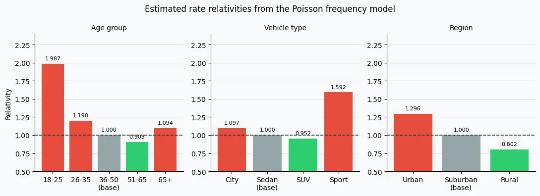
# Rate relativities from the frequency model
freq_relativities = np.exp(freq_model.params).rename('Frequency Relativity')
print(freq_relativities.round(3))
Intercept                                    0.083
C(age_group, ...)[T.18-25]                   1.987
C(age_group, ...)[T.26-35]                   1.198
C(age_group, ...)[T.51-65]                   0.903
C(age_group, ...)[T.65+]                     1.094
C(vehicle_type, ...)[T.city]                 1.097
C(vehicle_type, ...)[T.sport]                1.592
C(vehicle_type, ...)[T.suv]                  0.952
C(region, ...)[T.rural]                      0.802
C(region, ...)[T.urban]                      1.296
The intercept 0.083 is the base annual claim rate. The 18-25 relativity of 1.987 means ~2× the claim frequency of the 36-50 base group.
11) Python: Gamma severity model
The severity model is fitted on the claims-only subset. We use sm.families.Gamma with an explicit Log() link:
# ── SEVERITY MODEL ────────────────────────────────────────────────────────
claims_only = data[data['claim_count'] > 0].copy()

sev_formula = (
    "claim_amount ~ "
    "C(age_group, Treatment('36-50')) + "
    "C(vehicle_type, Treatment('sedan')) + "
    "C(region, Treatment('suburban'))"
)

sev_model = smf.glm(
    formula=sev_formula,
    data=claims_only,
    family=sm.families.Gamma(link=sm.families.links.Log())
).fit()

# Rate relativities from the severity model
sev_relativities = np.exp(sev_model.params).rename('Severity Relativity')
print(sev_relativities.round(3))
12) Interpreting rate relativities
A relativity above 1 means the segment is riskier than the base; below 1 means it is safer. To visualise:
fig, axes = plt.subplots(1, 2, figsize=(12, 4))

age_labels = ['18-25', '26-35', '51-65', '65+']

# Frequency relativities by age
f_age = [np.exp(freq_model.params.get(f"C(age_group, Treatment('36-50'))[T.{a}]", 0))
         for a in age_labels]
axes[0].bar(age_labels, f_age, color=['#e74c3c' if v > 1.1 else '#2ecc71' for v in f_age])
axes[0].axhline(1.0, color='black', linestyle='--', linewidth=1)
axes[0].set_title('Frequency Relativities: Age Group')
axes[0].set_ylabel('Relativity')

# Severity relativities by age
s_age = [np.exp(sev_model.params.get(f"C(age_group, Treatment('36-50'))[T.{a}]", 0))
         for a in age_labels]
axes[1].bar(age_labels, s_age, color=['#e74c3c' if v > 1.05 else '#2ecc71' for v in s_age])
axes[1].axhline(1.0, color='black', linestyle='--', linewidth=1)
axes[1].set_title('Severity Relativities: Age Group')
axes[1].set_ylabel('Relativity')

plt.tight_layout()
plt.show()
Notice that the frequency effect for young drivers is much larger than the severity effect: young drivers have accidents more often, but the per-accident cost is only moderately higher. This decomposition directly informs underwriting decisions: targeted telematics programmes, for example, primarily address frequency.
13) Auto tariff segmentation
Once both models are fitted, we compute the pure premium for every policy and aggregate into a tariff grid:
# ── PURE PREMIUM ─────────────────────────────────────────────────────────
# Predicted frequency rate (per year)
data['pred_freq'] = freq_model.predict(data) / data['exposure']

# Predicted severity (for all rows: even non-claimants, for the expectation)
data['pred_sev'] = sev_model.predict(data)

# Pure premium
data['pure_premium'] = data['pred_freq'] * data['pred_sev']

# ── TARIFF GRID: age_group × vehicle_type ────────────────────────────────
tariff = (
    data.groupby(['age_group', 'vehicle_type'])['pure_premium']
    .mean()
    .unstack('vehicle_type')
    .reindex(['18-25', '26-35', '36-50', '51-65', '65+'])
    .round(0)
)

print("Pure Premium Tariff Grid (£/year)")
print(tariff.to_string())
Pure Premium Tariff Grid (£/year)
vehicle_type   city  sedan    suv  sport
age_group
18-25           232    211    239    504
26-35           141    128    145    305
36-50           118    107    121    254
51-65           106     96    109    228
65+             123    112    127    267
A young driver (18-25) of a sports car pays a pure premium roughly 4.7× higher than a 51-65 sedan driver: the combined effect of high frequency and high severity relativities.
To convert to a gross premium, apply a combined ratio loading:
EXPENSE_RATIO   = 0.25  # 25% for acquisition, admin, claims handling
PROFIT_LOADING  = 0.05  # 5% target technical profit

data['gross_premium'] = data['pure_premium'] / (1 - EXPENSE_RATIO - PROFIT_LOADING)

# Gross tariff grid
gross_tariff = (
    data.groupby(['age_group', 'vehicle_type'])['gross_premium']
    .mean().unstack().round(0)
)
print(gross_tariff)
14) Model diagnostics
Fitting a GLM is only half the job. Before promoting a model to production, validate it:
- Residual deviance / df. Should be close to 1 for a well-specified model. A value of 2–3 for Poisson signals overdispersion; consider quasi-Poisson or Negative Binomial.
- Pearson chi-square statistic. $\chi^2_P / \text{df} \approx 1$ for Poisson. Available in
model.pearson_chi2 / model.df_resid. - AIC / BIC. Use for variable selection: lower is better. Compare nested models with the likelihood-ratio test (
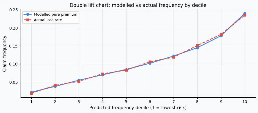
model.compare_lr_test(restricted_model)). - Double lift chart. Rank policies by modelled pure premium, group into deciles, compare modelled vs actual loss ratio per decile. A good model should show a monotone ordering.
- Gini coefficient. Measures the model's ability to discriminate between high- and low-risk policies. Calculated from the lift curve.
# ── QUICK DIAGNOSTICS ────────────────────────────────────────────────────
print("=== FREQUENCY MODEL ===")
print(f"Null deviance    : {freq_model.null_deviance:.1f}")
print(f"Residual deviance: {freq_model.deviance:.1f}")
print(f"AIC              : {freq_model.aic:.1f}")
pearson_freq = freq_model.pearson_chi2 / freq_model.df_resid
print(f"Pearson chi2/df  : {pearson_freq:.3f}  (1.0 = perfect for Poisson)")

print("\n=== SEVERITY MODEL ===")
print(f"Null deviance    : {sev_model.null_deviance:.1f}")
print(f"Residual deviance: {sev_model.deviance:.1f}")
print(f"AIC              : {sev_model.aic:.1f}")
pearson_sev = sev_model.pearson_chi2 / sev_model.df_resid
print(f"Pearson chi2/df  : {pearson_sev:.3f}  (1.0 = perfect for Gamma)")
# ── DOUBLE LIFT CHART ────────────────────────────────────────────────────
data['pp_decile'] = pd.qcut(data['pure_premium'], q=10, labels=False)

lift = data.groupby('pp_decile').agg(
    modelled_pp=('pure_premium', 'mean'),
    actual_loss=('claim_amount', lambda x: x.sum() / data.loc[x.index, 'exposure'].sum())
).reset_index()

plt.figure(figsize=(8, 4))
plt.plot(lift['pp_decile'] + 1, lift['modelled_pp'], 'o-', label='Modelled Pure Premium', color='#007bff')
plt.plot(lift['pp_decile'] + 1, lift['actual_loss'], 's--', label='Actual Loss Rate', color='#e74c3c')
plt.xlabel('Pure Premium Decile')
plt.ylabel('£ per year')
plt.title('Double Lift Chart')
plt.legend()
plt.grid(True, alpha=0.3)
plt.tight_layout()
plt.show()
15) Glossary
- Claim frequency: expected number of claims per unit exposure. Modelled with Poisson GLM.
- Claim severity: expected cost per claim. Modelled with Gamma GLM on claims-only data.
- Pure premium: expected aggregate loss per unit exposure = frequency × severity.
- Rate relativity: multiplicative factor for a variable level; equal to $e^{\hat{\beta}_j}$.
- Exposure: the time period (in years) a policy is at risk. Used as an offset in the frequency model.
- Link function: $g(\mu)$ that connects the expected response to the linear predictor. Log link gives multiplicative relativities.
- Deviance: twice the difference in log-likelihood between the saturated model and the fitted model. Lower is better.
- Overdispersion: variance exceeds the mean; indicates the Poisson assumption may not hold.
- Tweedie distribution: compound Poisson-Gamma distribution; models aggregate losses directly. Useful shortcut but less interpretable.
- Bonus-malus: merit rating system that adjusts premiums based on claim history. Typically enters as a rating factor in the GLM.
- IRLS: Iteratively Reweighted Least Squares; the numerical algorithm used to fit GLM parameters via MLE.
- Gini coefficient: model discrimination metric; 0 = no discrimination, 1 = perfect discrimination.
16) References
- Anderson, D., Feldblum, S., Modlin, C., Schirmacher, D., Schirmacher, E., & Thandi, N. (2007). A Practitioner's Guide to Generalized Linear Models. Casualty Actuarial Society.
- De Jong, P., & Heller, G. Z. (2008). Generalized Linear Models for Insurance Data. Cambridge University Press.
- Ohlsson, E., & Johansson, B. (2010). Non-Life Insurance Pricing with Generalized Linear Models. Springer.
- McCullagh, P., & Nelder, J. A. (1989). Generalized Linear Models (2nd ed.). Chapman & Hall.
- Frees, E. W. (2009). Regression Modeling with Actuarial and Financial Applications. Cambridge University Press.
- statsmodels GLM documentation.
17) FAQ
Q1. Why not just use a random forest or XGBoost for pricing?
Tree-based models can achieve better predictive accuracy on held-out data, but they are hard to interpret, difficult to audit, and regulators in most markets require transparent pricing models. GLMs give you exact rate relativities per factor, which are essential for rate filing, underwriting guidelines, and Solvency II documentation. Many insurers use gradient boosting to suggest factor structure, then refit a GLM on that structure.
Q2. How do I handle continuous variables like vehicle age or driver age in years?
Options: (1) group into bands and treat as categorical: simple and interpretable; (2) use a spline basis (e.g., bs(age, df=4) in R or manually via patsy in Python): smoother but harder to audit; (3) fit a piecewise-linear term. For regulatory filings, banded categorical variables are the most defensible.
Q3. My Pearson chi-square / df is 3.2 for the Poisson model. What should I do?
Overdispersion of that magnitude suggests either a missing important variable (try adding vehicle age, annual mileage, or bonus-malus level), or an intrinsically overdispersed process. Fit a Negative Binomial GLM (sm.families.NegativeBinomial()) which adds a free dispersion parameter, or use quasi-Poisson (scale deviance by the estimated dispersion) as a quick correction to standard errors.
Q4. How do I validate the model on a hold-out set?
Split by policy year: train on years $t-3$ to $t-1$, validate on year $t$. Compute the Gini coefficient on the validation set: rank policies by predicted pure premium, plot the cumulative proportion of actual losses against cumulative proportion of policies (ordered by risk). The area between the Lorenz curve and the diagonal, doubled, is the Gini. A well-calibrated auto pricing GLM typically achieves Gini 0.25–0.45.
Q5. Can I include interactions between factors?
Yes. Add an interaction term with the : or * operator in the patsy formula: C(age_group) : C(vehicle_type). Each interaction cell needs sufficient claims volume to be estimated reliably: a rule of thumb is at least 50–100 claims per cell. Sparse cells require smoothing (credibility weighting) or regularisation (Elastic Net GLM via glmnet in R, or sklearn with Poisson loss in Python).
Comments