Support Vector Machines: Understanding the Math Behind SVM
Support Vector Machines (SVMs) are one of those algorithms every data scientist hears about early on… but the math can feel intimidating. The good news: once you understand “maximize the margin” and the idea of the kernel trick, most of SVMs fall into place. This article walks slowly through the geometry, the optimization problem, hard vs soft margin, hinge loss, dual formulation, kernels (linear, polynomial, RBF), plus hands-on scikit-learn code and practical tips for when SVMs shine (and when they don’t).
1. Intuition: A Straight Line That Plays It Safe
Suppose you have two classes of points in 2D (say, red and blue). There are many possible straight lines that separate them. Which one is “best”?
The SVM answer: choose the line that leaves the largest possible gap (margin) between the two classes. Intuitively, if you later see slightly noisy or shifted data, that line is more robust — it’s not hugging any particular point too tightly.
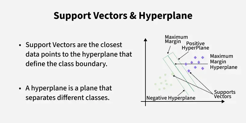
A linear SVM finds the separating line that maximizes the margin between the closest points (support vectors).
In higher dimensions, that line becomes a hyperplane. The points that lie closest to this hyperplane are the support vectors. They “support” the solution: if you removed other points far away, the boundary wouldn’t move; if you removed a support vector, it might.
2. Hard-Margin SVM: Perfect Separation with Maximum Margin
Let’s start with the ideal case: the data is perfectly linearly separable — we can draw a straight hyperplane that gets all labels right.
A linear classifier has the form:
The prediction is:
For correctly classified points with labels \( y_i \in \{+1, -1\} \):
2.1 Margin definition
The (geometric) distance from a point \( \mathbf{x}_i \) to the hyperplane \( \mathbf{w}^\top \mathbf{x} + b = 0 \) is:
For the nearest points (support vectors) we enforce:
Under this scaling convention, the margin becomes:
So, maximizing the margin is equivalent to minimizing \( \|\mathbf{w}\| \).
2.2 Hard-margin optimization problem
Putting it all together, the hard-margin SVM solves:
This is a quadratic programming problem: a quadratic objective with linear constraints.
3. Soft Margin & Hinge Loss: Being Okay with a Few Mistakes
In practice, data is messy. Outliers exist. If you insist on perfect separation, you might end up with a crazy, almost vertical hyperplane that overfits.
Soft-margin SVM introduces slack variables \( \xi_i \ge 0 \) that allow some violations:
The new optimization problem becomes:
- \( \frac{1}{2}\|\mathbf{w}\|^2 \): keep the margin large (simpler boundary).
- \( C \sum \xi_i \): penalize margin violations (misclassifications / points inside the margin).
3.1 Hinge loss view
Soft-margin SVMs can also be written using the hinge loss:
The regularized risk minimization form becomes:
Compare with logistic regression (log loss). Both are linear classifiers with different loss functions and regularization styles.
4. Dual Form & Why Only Support Vectors Matter
The SVM can also be expressed in a dual form using Lagrange multipliers. This is where the kernel trick will show up nicely.
4.1 Lagrangian setup (high level)
We introduce multipliers \( \alpha_i \ge 0 \) for each constraint \( y_i(\mathbf{w}^\top \mathbf{x}_i + b) \ge 1 - \xi_i \), and others for \( \xi_i \ge 0 \). After some algebra (skipping the full derivation here), the dual problem for the soft-margin SVM becomes:
The optimal weights can be recovered from the multipliers:
Notice that only points with \( \alpha_i^\star > 0 \) matter in this sum. These are the support vectors. Everyone else has \( \alpha_i = 0 \) and doesn’t influence the final classifier.
5. The Kernel Trick: Nonlinear Boundaries Without Mapping Explicitly
What if the classes are not linearly separable in the original feature space? The classic SVM move: map the inputs into a higher-dimensional feature space where a linear separator does exist.
But computing that mapping explicitly can be expensive or even infinite-dimensional. The kernel trick says:
- We never need \( \phi(\mathbf{x}) \) explicitly.
- We only need inner products \( \phi(\mathbf{x}_i)^\top \phi(\mathbf{x}_j) \).
- Define a function \( K(\mathbf{x}_i, \mathbf{x}_j) \) that acts like that inner product.
In the dual objective, inner products appear as \( \mathbf{x}_i^\top \mathbf{x}_j \). We replace them by a kernel:
5.1 Common kernels
- Linear kernel \( K(\mathbf{x}, \mathbf{z}) = \mathbf{x}^\top \mathbf{z} \) Good baseline; equivalent to a linear SVM in the original space.
- Polynomial kernel \( K(\mathbf{x}, \mathbf{z}) = (\gamma\,\mathbf{x}^\top \mathbf{z} + r)^d \) Useful when interactions between features matter but you don’t want to manually create polynomial features.
- RBF / Gaussian kernel \( K(\mathbf{x}, \mathbf{z}) = \exp(-\gamma \|\mathbf{x} - \mathbf{z}\|^2) \) Very popular. Allows very flexible, nonlinear boundaries. Hyperparameter \( \gamma \) controls how “local” the influence of a point is.
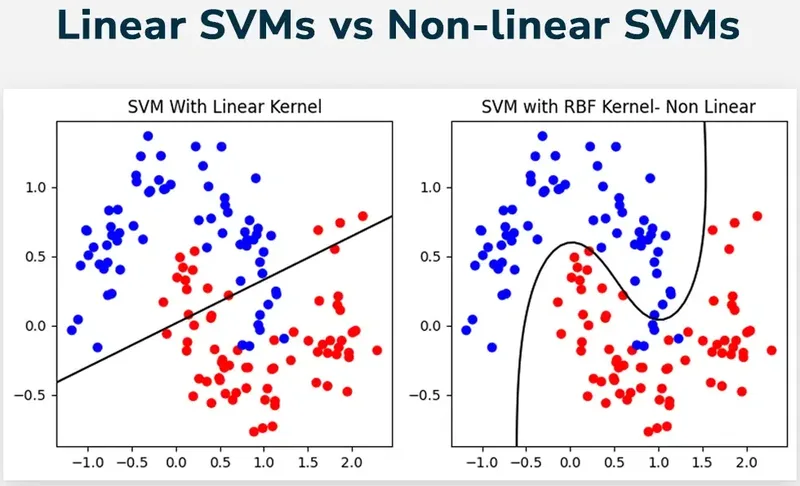
With an RBF kernel, the decision boundary can wrap around clusters in complex ways, even though the SVM is still linear in the implicit feature space.
6. Tiny 2D Example: Max Margin by Hand (Very Roughly)
Consider a toy dataset in 2D:
- Class +1: \( (2, 2), (2, 3) \)
- Class −1: \( (0, 0), (1, 0) \)
Plotting this, you can see a roughly diagonal separation. We won’t solve the full QP here, but conceptually:
- Try a candidate line, e.g., \( x_2 = x_1 + 0.5 \Rightarrow \mathbf{w} = (-1, 1), b = 0.5 \).
- Check constraints \( y_i(\mathbf{w}^\top \mathbf{x}_i + b) \ge 1 \); rescale \( \mathbf{w}, b \) to meet the margin conditions.
- The support vectors will be the closest points to the boundary on each side.
SVM solvers do this systematically using convex optimization. The example is just to emphasize: the algorithm is really just geometry + optimization.
7. Hands-On: SVM in Python with scikit-learn
Let’s train an SVM on a simple nonlinear dataset using the RBF kernel.
import numpy as np
import matplotlib.pyplot as plt
from sklearn.datasets import make_moons
from sklearn.svm import SVC
from sklearn.metrics import accuracy_score, confusion_matrix

# 1) Data: two interleaving half circles
X, y = make_moons(noise=0.2, random_state=42)

# 2) Train/test split
from sklearn.model_selection import train_test_split
X_train, X_test, y_train, y_test = train_test_split(
    X, y, test_size=0.3, random_state=42, stratify=y
)

# 3) SVM with RBF kernel
clf = SVC(kernel="rbf", C=1.0, gamma=0.5)  # try different C, gamma
clf.fit(X_train, y_train)

# 4) Evaluation
y_pred = clf.predict(X_test)
print("Accuracy:", accuracy_score(y_test, y_pred))
print("Confusion matrix:\n", confusion_matrix(y_test, y_pred))

# 5) Plot decision boundary
def plot_decision_boundary(model, X, y):
    x_min, x_max = X[:,0].min() - 0.5, X[:,0].max() + 0.5
    y_min, y_max = X[:,1].min() - 0.5, X[:,1].max() + 0.5
    xx, yy = np.meshgrid(
        np.linspace(x_min, x_max, 300),
        np.linspace(y_min, y_max, 300)
    )
    grid = np.c_[xx.ravel(), yy.ravel()]
    zz = model.predict(grid).reshape(xx.shape)

    plt.contourf(xx, yy, zz, alpha=0.3, cmap="coolwarm")
    plt.scatter(X[:,0], X[:,1], c=y, cmap="coolwarm", edgecolors="k")
    plt.title("SVM with RBF kernel")
    plt.show()

plot_decision_boundary(clf, X, y)
The decision boundary will curve to separate the two moon-shaped clusters. Play with:
C: higher → more complex boundary, more risk of overfitting.gamma: higher → each point’s influence is more local, leading to wigglier boundaries.
kernel="rbf", C=1.0, gamma="scale" (the
scikit-learn default).
7.1 Multi-class SVM in scikit-learn
SVMs are inherently binary classifiers, but they can be extended to multi-class via:
- One-versus-rest (OvR): train one classifier per class vs all others.
- One-versus-one (OvO): train one classifier for each pair of classes.
scikit-learn’s SVC handles this automatically:
from sklearn import datasets
from sklearn.preprocessing import StandardScaler
from sklearn.pipeline import make_pipeline

# 3-class iris dataset
iris = datasets.load_iris()
X_iris, y_iris = iris.data, iris.target

svm_clf = make_pipeline(
    StandardScaler(),
    SVC(kernel="rbf", C=1.0, gamma="scale", decision_function_shape="ovr")
)
svm_clf.fit(X_iris, y_iris)
print("Iris training accuracy:", svm_clf.score(X_iris, y_iris))
8. Hyperparameters: C and Gamma Without the Magic
The two most important knobs for an RBF SVM are \( C \) and \( \gamma \).
8.1 Regularization parameter \( C \)
- High \( C \): – Strongly penalizes misclassifications – Tries to classify every training point correctly – Risk of overfitting, especially with noisy labels.
- Low \( C \): – Allows more violations of the margin – Smoother, more regularized boundary – Better generalization when data is noisy.
8.2 Kernel width \( \gamma \) (for RBF)
In the RBF kernel:
- Small \( \gamma \): kernel varies slowly → each point influences a large region → smoother boundary.
- Large \( \gamma \): kernel is very peaked → each point influences only a small region → highly flexible, may overfit.
In practice, we tune \( C \) and \( \gamma \) with cross-validation, usually with a grid search in log-space (e.g., \( C \in \{0.1, 1, 10, 100\} \), \( \gamma \in \{0.01, 0.1, 1, 10\} \)).
from sklearn.model_selection import GridSearchCV

param_grid = {
    "svc__C": [0.1, 1, 10, 100],
    "svc__gamma": [0.01, 0.1, 1, 10]
}

pipe = make_pipeline(
    StandardScaler(),
    SVC(kernel="rbf")
)

grid = GridSearchCV(pipe, param_grid, cv=5, n_jobs=-1)
grid.fit(X_train, y_train)

print("Best params:", grid.best_params_)
print("Best CV score:", grid.best_score_)
9. Variants: SVR, One-Class SVM & Multi-class Strategies
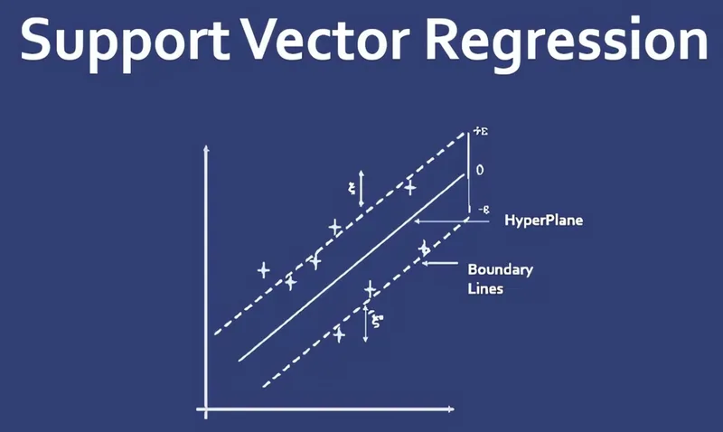
9.1 Support Vector Regression (SVR)
SVMs aren’t just for classification. Support Vector Regression (SVR) adapts the idea to regression:
- Instead of a margin between classes, we use an \(\varepsilon\)-insensitive tube around the regression function.
- Points inside the tube incur zero loss; only points outside contribute.
The loss is:
from sklearn.svm import SVR

svr = SVR(kernel="rbf", C=1.0, epsilon=0.1, gamma="scale")
svr.fit(X_train_reg, y_train_reg)
y_pred_reg = svr.predict(X_test_reg)
9.2 One-Class SVM (Anomaly Detection)
One-class SVM tries to learn the “region” where the data lives, treating anything outside as an anomaly.
scikit-learn provides OneClassSVM for this:
from sklearn.svm import OneClassSVM

ocs = OneClassSVM(kernel="rbf", nu=0.05, gamma="scale")
ocs.fit(X_train_normal)
anomaly_scores = ocs.predict(X_test)  # -1 = outlier, +1 = inlier
This is useful for fraud detection, monitoring systems, or any setting where “normal” is well-defined and anomalies are rare.
10. When to Use SVM (and When Not To)
10.1 Strengths
- Strong performance on small to medium-sized tabular datasets, especially with good feature engineering.
- Robust to high-dimensional spaces (e.g., text classification with bag-of-words or TF-IDF features).
- Well-defined optimization problem — convex, global optimum.
- Interpretable geometry: margin, support vectors, influence of C and kernels.
10.2 Weaknesses
- Training time can be high for very large datasets (hundreds of thousands or millions of points).
- Memory usage scales with the number of support vectors.
- Hyperparameter tuning (C, kernel, gamma) can be sensitive and expensive.
- Less popular for raw images/audio now that deep nets dominate there.
11. Recommended Video: StatQuest on SVM
If you prefer animations and step-by-step visuals, this StatQuest video is an excellent complement to this article:
12. References & Further Reading
- Vapnik, V. N. (1998). Statistical Learning Theory. Wiley.
- Cortes, C., & Vapnik, V. (1995). Support-Vector Networks. Machine Learning, 20(3).
- Hastie, T., Tibshirani, R., & Friedman, J. (2009). The Elements of Statistical Learning. Ch. 12, “Support Vector Machines”.
- scikit-learn documentation: Support Vector Machines.
- Wikipedia: Support Vector Machine, Kernel method, Hinge loss.
Author's Perspective
Teaching the math behind SVMs has been one of the most rewarding challenges in my experience as an educator. I have seen students struggle with the Lagrangian dual formulation and KKT conditions for weeks, only to have everything click the moment they visualize the geometric intuition: you are simply looking for the widest possible street between two classes of points, and the support vectors are the buildings lining that street. Once that picture settles in, the optimization framework stops feeling abstract and starts feeling inevitable.
One thing I always tell my students is that SVMs taught me more about mathematical optimization than any other algorithm. The journey from the primal problem to the dual, the role of slack variables in the soft-margin case, and the kernel trick as implicit feature mapping -- these concepts appear everywhere in machine learning, from logistic regression to modern neural network theory. Mastering them through SVMs gives you a toolkit that transfers far beyond this single algorithm.
In an era dominated by deep learning, people often ask whether SVMs still matter. From my practical experience, the answer is a clear yes for specific use cases: small datasets where you cannot afford to overfit, high-dimensional problems like text classification with TF-IDF features, and any domain where model interpretability and mathematical guarantees on the margin matter. I have seen SVMs outperform neural networks in production medical diagnostics pipelines where training data was limited to a few hundred labeled samples. The right tool depends on the problem, and SVMs remain a sharp tool in the practitioner's kit.
Comments