Top 10 Machine Learning Algorithms Explained — Intuition, Math, Code, and Use Cases
Choosing the right algorithm is half the battle in machine learning. This gently technical deep dive explains the Top 10 ML algorithms with plain-English intuition, key equations, Python snippets, and realistic use cases. We also add ensembles like XGBoost/AdaBoost, common pitfalls, a mini history, and interview questions—so beginners can follow, and practitioners still learn something new.
Why these 10? (and how to pick fast)
Plain English. The algorithms below are the most reused across analytics, data products, and ML engineering. They’re battle-tested, well-understood, and widely implemented. Learn these first, then specialize.
| Algorithm | Type | Strength | Watch out for |
|---|---|---|---|
| Linear Regression | Supervised (regression) | Fast, interpretable coefficients | Outliers, multicollinearity |
| Logistic Regression | Supervised (classification) | Calibrated probs, simple baseline | Nonlinear boundaries |
| Decision Tree | Supervised | Human-readable rules | Overfitting without pruning |
| Random Forest | Supervised (ensemble) | Strong baseline, robust | Less interpretable than single tree |
| SVM | Supervised | Clear margins; kernels for nonlinearity | Scaling, kernel tuning |
| k-NN | Supervised (lazy) | Simple, nonparametric | Curse of dimensionality |
| Naive Bayes | Supervised (probabilistic) | Fast, decent text baseline | Feature independence assumption |
| k-Means | Unsupervised (clustering) | Fast, widely used | Spherical clusters; init sensitivity |
| PCA | Unsupervised (DR) | Noise reduction, visualization | Linear components only |
| Neural Networks | Supervised / self-supervised | State-of-the-art representation learning | Compute, data, tuning |
1) Linear Regression
Intuition. Predict a number as a weighted sum of features. Like mixing sliders on a soundboard: each feature’s coefficient says how much it nudges the prediction.
Closed form (OLS): \(\hat{\boldsymbol{\beta}}=(X^\top X)^{-1}X^\top y\). In practice, prefer numerically stable solvers (QR/SVD) or gradient methods.
# Linear Regression with scikit-learn
import numpy as np
from sklearn.linear_model import LinearRegression
from sklearn.metrics import r2_score, mean_squared_error

rng = np.random.default_rng(0)
X = rng.normal(size=(200, 3))
true_beta = np.array([2.0, -1.0, 0.5])
y = 1.3 + X @ true_beta + rng.normal(scale=0.5, size=200)

model = LinearRegression().fit(X, y)
y_pred = model.predict(X)
print("Coefficients:", model.coef_)
print("R^2:", r2_score(y, y_pred), "RMSE:", mean_squared_error(y, y_pred, squared=False))
2) Logistic Regression
Intuition. Linear scores passed through a sigmoid give probabilities for binary outcomes.
Loss: negative log-likelihood (a.k.a. logistic loss). Regularization (L2/L1) helps avoid overfitting, improves conditioning.
# Logistic Regression
from sklearn.datasets import make_classification
from sklearn.linear_model import LogisticRegression
from sklearn.metrics import roc_auc_score

X, y = make_classification(n_samples=800, n_features=8, random_state=0)
clf = LogisticRegression(max_iter=1000).fit(X, y)
p = clf.predict_proba(X)[:,1]
print("AUC:", roc_auc_score(y, p))
3) Decision Trees
Intuition. Split the feature space into rectangles by asking yes/no questions (“Is price < 250k?”). Leaves are predictions; paths are human-readable rules.
Pick the split that reduces impurity the most. Risk: overfitting—mitigate via max depth, min samples, cost-complexity pruning.
# Decision Tree
from sklearn.tree import DecisionTreeClassifier, export_text
tree = DecisionTreeClassifier(max_depth=4, random_state=0).fit(X, y)
print(export_text(tree, feature_names=[f"x{i}" for i in range(X.shape[1])]))
4) Random Forests
Intuition. Many de-correlated trees vote together. Bagging reduces variance; random feature selection further de-correlates trees.
# Random Forest
from sklearn.ensemble import RandomForestClassifier
rf = RandomForestClassifier(n_estimators=300, oob_score=True, random_state=0).fit(X, y)
print("OOB score:", rf.oob_score_)
5) Support Vector Machines
Intuition. Find the separating hyperplane with the largest margin. With kernels, implicitly map data to a space where separation is easier.
Tips: scale features; tune \(C\) and kernel parameters (e.g., RBF \(\gamma\)). Works well on moderate-sized datasets.
# SVM (RBF)
from sklearn.svm import SVC
from sklearn.preprocessing import StandardScaler
from sklearn.pipeline import make_pipeline

svm = make_pipeline(StandardScaler(), SVC(kernel="rbf", C=2.0, gamma="scale", probability=True))
svm.fit(X, y)
6) k-Nearest Neighbors
Intuition. “You are who your neighbors are.” Classification or regression from the average of the k closest points in feature space.
# k-NN
from sklearn.neighbors import KNeighborsClassifier
knn = KNeighborsClassifier(n_neighbors=7, weights="distance").fit(X, y)
7) Naive Bayes
Intuition. Apply Bayes’ rule with a strong independence assumption to get simple, fast probabilistic classifiers—great for text.
Types: Gaussian, Multinomial, Bernoulli. Use cases: spam filtering, quick baselines for NLP. Watch: correlated features break the assumption.
# Multinomial Naive Bayes (text-like)
from sklearn.naive_bayes import MultinomialNB
from sklearn.feature_extraction.text import CountVectorizer

docs = ["great service", "bad product", "excellent quality", "terrible experience"]
y_text = [1, 0, 1, 0]
vec = CountVectorizer().fit(docs)
X_text = vec.transform(docs)

nb = MultinomialNB().fit(X_text, y_text)
8) k-Means Clustering
Intuition. Repeatedly assign points to the nearest centroid, then recompute centroids. Finds compact, spherical-ish clusters.
Tips: standardize features; try different \(K\) (elbow, silhouette); use k-means++ init.
# k-Means
from sklearn.cluster import KMeans
from sklearn.metrics import silhouette_score

km = KMeans(n_clusters=4, init="k-means++", random_state=0).fit(X)
labels = km.labels_
print("Silhouette:", silhouette_score(X, labels))
9) Principal Component Analysis (PCA)
Intuition. Rotate the data to directions of maximum variance; keep only the top components to compress noise while preserving structure.
Use cases: visualization (2D/3D), preprocessing, denoising. Note: linear method—nonlinear structure may need t-SNE/UMAP/kPCA.
# PCA
from sklearn.decomposition import PCA
pca = PCA(n_components=2).fit(X)
Z = pca.transform(X)
print("Explained variance ratio:", pca.explained_variance_ratio_)
10) Neural Networks (MLP → CNNs → Transformers)
Intuition. Stack layers of linear transforms + nonlinear activations to learn flexible functions. Depth and width control capacity.
Use cases: images (CNNs), sequences (RNNs/LSTMs), language (Transformers). Needs: data, compute, regularization (dropout, weight decay), good optimization (AdamW, schedulers).
# Minimal MLP in PyTorch
import torch, torch.nn as nn, torch.optim as optim
class MLP(nn.Module):
    def __init__(self, d_in, d_h, d_out):
        super().__init__()
        self.net = nn.Sequential(
            nn.Linear(d_in, d_h), nn.ReLU(),
            nn.Linear(d_h, d_out)
        )
    def forward(self, x): return self.net(x)

X_t = torch.tensor(X, dtype=torch.float32)
y_t = torch.tensor(y, dtype=torch.float32).view(-1,1)
mlp = MLP(d_in=X.shape[1], d_h=64, d_out=1)
opt = optim.AdamW(mlp.parameters(), lr=1e-3, weight_decay=1e-2)
loss_fn = nn.MSELoss()

for _ in range(400):
    opt.zero_grad()
    pred = mlp(X_t)
    loss = loss_fn(pred, y_t)
    loss.backward(); opt.step()
Bonus: Ensembles (XGBoost, AdaBoost, Gradient Boosting)
Why ensembles win. Combine many weak learners (typically shallow trees) to get a strong learner. Boosting adds models sequentially, focusing on previous mistakes.
AdaBoost (Adaptive Boosting)
Reweights samples: misclassified points get higher weights. Final prediction is a weighted vote.
Gradient Boosting (incl. XGBoost/LightGBM)
Fit the next tree to the negative gradient of the loss w.r.t. current predictions (i.e., to residuals). Regularization (shrinkage, subsampling) prevents overfitting.
# Gradient Boosting / XGBoost-like (scikit-learn)
from sklearn.ensemble import GradientBoostingClassifier
gb = GradientBoostingClassifier(n_estimators=300, learning_rate=0.05, max_depth=3, random_state=0).fit(X, y)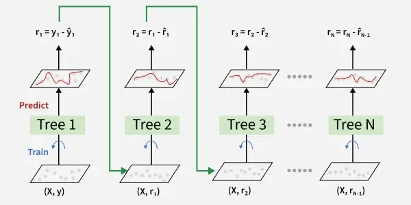
Mini History & Trends
Then → Now. We went from early statistical models (linear/logistic regression), to tree-based methods and kernels (SVM), to ensemble dominance (Random Forest, boosting), and now to representation learning with deep learning and Transformers handling images, speech, and language. On tabular data, boosting remains a strong baseline; on perceptual tasks, deep nets are king; and for interpretability, linear models and trees still shine.
Interview-Style Questions (with short answers)
- Q: Why prefer Logistic Regression over SVM sometimes? A: Calibrated probabilities, simpler/faster baseline, easier to interpret coefficients.
- Q: Gini vs Entropy in trees? A: Both measure impurity; Gini is slightly faster; they usually choose similar splits.
- Q: When does k-NN fail? A: High dimensions (distances become uninformative), unscaled features, large datasets (slow lookup).
- Q: PCA vs t-SNE? A: PCA is linear, fast, preserves global variance; t-SNE is nonlinear, good for 2D cluster visualization but distorts global structure.
- Q: Why are ensembles strong? A: Averaging reduces variance; boosting reduces bias by focusing on errors.
Common Pitfalls & Diagnostics
- Data leakage: Don’t compute scalers/PCA on full data. Fit on train only; apply to validation/test.
- Imbalanced classes: Use stratified CV, class weights, threshold tuning, PR-AUC, and focal/weighted losses.
- Overfitting trees: Restrict depth, min samples; use ensembles with regularization.
- Poor scaling: Standardize for SVM/k-NN/PCA/logistic; trees/forests don’t require scaling.
- Bad metrics: Accuracy is misleading on imbalance; prefer ROC-AUC/PR-AUC/F1, MCC, calibration.
- Tabular baseline: Random Forest or Gradient Boosting (+ simple feature engineering).
- Need probabilities & interpretability: Logistic Regression with regularization + calibration.
- Small data, nonlinear boundary: SVM (RBF), after scaling.
- Clustering customers: k-Means after standardization; validate with silhouette.
- Dimensionality/tSNE plots: PCA → t-SNE/UMAP.
- Images/text/audio: Neural Networks; start with pretrained models.
References & Further Reading
- Machine learning — Wikipedia
- scikit-learn User Guide (great API docs + tutorials)
- Hastie, Tibshirani, Friedman. The Elements of Statistical Learning.
- Goodfellow, Bengio, Courville. Deep Learning.
- Breiman, L. “Random Forests.” Machine Learning (2001).
- Friedman, J. “Greedy Function Approximation: A Gradient Boosting Machine.” (2001).
Comments