The Complete Beginner’s Guide to Gradient Descent (Beginner-Friendly & Detailed)

Gradient descent is the workhorse behind modern machine learning. In this guide we go slow and logical: first the goal and the idea of a loss, then the gradient and the famous one-line update, then safe learning-rate choices with tiny numeric examples and visuals. Only after that do we introduce practical variants (mini-batches, momentum, Adam) with clear definitions and code you can run.

---

1) Objective: what are we minimizing?

---

Plain English. We want the model to make fewer mistakes. We turn “mistakes” into a number called the loss. Lower is better.

• Regression: Mean Squared Error (MSE) \(\; \frac{1}{n}\sum_i (y_i-\hat y_i)^2\).
• Classification: Cross-Entropy (log loss).
• Language models: also Cross-Entropy—predicting the next token.

---

2) Gradient: which way is downhill?

---

Idea. The gradient points to the direction of steepest increase. So we walk the opposite way to reduce the loss fast.

---

3) The update rule (and the famous minus sign)

---

At step \(t\), with learning rate \(\eta\), take a small step opposite the gradient:

Why minus? Gradients point uphill; we want downhill.

---

4) Learning rate: how big should the step be?

---

Heuristic that works: start small, increase until the loss gets bouncy, then back off a bit.

• LR finder: raise \(\eta\) exponentially during a short run; pick the highest \(\eta\) before loss spikes, then divide by 3–10.
• Schedulers: warmup (start small), step decay, cosine decay—helpful once basics work.

---

5) Tiny 1D example (feel it numerically)

---

import numpy as np
def f(w):    return (w-3)**2
def grad(w): return 2*(w-3)

w, eta = 10.0, 0.1
for step in range(12):
    w -= eta * grad(w)
    print(f"step {step:2d}: w={w:6.3f}  loss={f(w):7.4f}")

Try \(\eta=1.2\) to see divergence—useful for intuition.

---

6) Visual intuition (contour map)

---

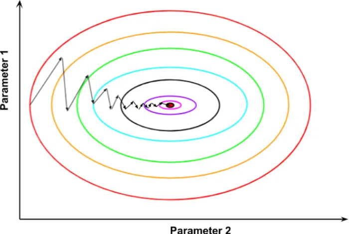
Reading the map. Lines are equal-loss contours; arrows point down (opposite gradient). In narrow valleys, steps can zig-zag—later we’ll fix this with momentum.

---

7) Scaling & conditioning (why standardize features)

---

When features have very different scales (e.g., age vs income), the loss “bowl” is stretched—some directions are steep, others flat. Gradient descent then zig-zags and needs a tiny \(\eta\). Standardizing inputs (zero mean, unit variance) makes the bowl rounder and training smoother.

---

8) Mini-batches & Stochastic Gradient Descent (now that GD is clear)

---

Full-batch gradient uses all \(n\) examples every step—accurate but slow. Stochastic GD uses one example—fast but very noisy. Mini-batch (e.g., 64–256 samples) balances speed and stability.

The noise in \(g_t\) can help escape saddles and poor local minima.

---

9) Momentum: keep some of your previous direction

---

Intuition. If you’ve been moving east, don’t instantly stop unless the slope forces you. Momentum damps zig-zags in narrow valleys.

Nesterov momentum peeks ahead a little before taking a step—often slightly better in practice.

---

10) Adam: momentum + adaptive per-parameter step sizes

---

Idea. Keep a moving average of gradients (like momentum) and also of squared gradients to scale each parameter’s step. Parameters with noisy gradients get smaller steps.

Popular defaults: \(\beta_1=0.9,\;\beta_2=0.999,\;\epsilon=10^{-8},\;\eta=10^{-3}\).

---

11) Hands-on: logistic regression trained with gradient descent

---

import numpy as np
from sklearn.datasets import make_classification
from sklearn.preprocessing import StandardScaler

# 1) Toy data
X, y = make_classification(n_samples=400, n_features=2, n_redundant=0,
                           n_clusters_per_class=1, random_state=0)
scaler = StandardScaler()
X = scaler.fit_transform(X)
X = np.c_[np.ones(len(X)), X]  # add bias column of ones

# 2) Model & helpers
w = np.zeros(X.shape[1])
def sigmoid(z): return 1/(1+np.exp(-z))
def loss(w):
    z = X @ w
    p = sigmoid(z)
    eps = 1e-9
    return -np.mean(y*np.log(p+eps) + (1-y)*np.log(1-p+eps))
def grad(w):
    z = X @ w
    p = sigmoid(z)
    return X.T @ (p - y) / len(y)

# 3) Train
eta = 0.2
for step in range(800):
    w -= eta*grad(w)
    if step % 100 == 0:
        print(f"step {step:4d}  loss={loss(w):.4f}")
print("weights:", w.round(3))

What you should see. Loss drops quickly then stabilizes; if it oscillates, lower \(\eta\); if it barely moves, increase \(\eta\) a bit.

---

12) Diagnosing training curves (simple rules)

---

• Loss barely moves: raise \(\eta\) (×2), standardize inputs, or try momentum \(0.9\).
• Loss explodes/NaN: lower \(\eta\); clip gradients; check for bad labels or log(0).
• Loss zig-zags: lower \(\eta\) slightly or add momentum; consider Adam.
• Train ↓, Val ↑: overfitting—use regularization (e.g., L2), reduce capacity, or early stopping.

---

13) Just enough theory (why steps reduce loss)

---

If the gradient is Lipschitz-continuous with constant \(L\) and \(0<\eta<2 /L\), each step decreases the loss unless you’re at a flat optimum:

For a 1D quadratic \(f(w)=\tfrac{a}{2}(w-w^\star)^2\), the update is \(w_{t+1}-w^\star=(1-\eta a)(w_t-w^\star)\). Convergence requires \(|1-\eta a|<1\Rightarrow 0<\eta<2/a\).

---

14) A tidy training loop (pseudo)

---

# Pseudo-code for a robust loop
init θ
optimizer = Adam(η=1e-3)         # or SGD+momentum once you’re comfortable
for epoch in range(E):
    for (x, y) in dataloader:    # mini-batches
        y_hat = model(x, θ)
        L     = loss(y_hat, y)
        g     = ∇θ L             # backprop computes this in frameworks
        θ     = optimizer.update(θ, g)
    # evaluate on validation set
    # adjust η with a scheduler if needed
    # early stop if validation loss worsens for K epochs

---

15) Video: 3Blue1Brown on gradient descent

---

---

16) Glossary (jargon → plain English)

---

• Loss function — number measuring how wrong the model is.
• Gradient — direction of steepest loss increase.
• Learning rate (η) — step size each update.
• Mini-batch — small subset used to estimate gradient quickly.
• Momentum — moving average of gradients to smooth updates.
• Adam — optimizer combining momentum + adaptive steps.
• Conditioning — how stretched the loss bowl is; bad conditioning slows GD.
• Scheduler — planned changes to \(\eta\) over training.

---

17) References & Further Reading

---

1. 3Blue1Brown. “Gradient descent, how neural networks learn.” (YouTube).
2. Ruder, S. “An Overview of Gradient Descent Optimization Algorithms.” arXiv:1609.04747.
3. Goodfellow, Bengio, Courville. Deep Learning, Ch. 8 (Optimization).
4. Wikipedia: Gradient Descent, Stochastic GD, Adam.

---

18) FAQ

---

Q1. How do I pick a learning rate without guessing?

Use an LR finder: start tiny, increase \(\eta\) exponentially, plot loss vs \(\eta\), pick the largest value before the curve turns up, then divide by 3–10.

Q2. Should I always use Adam?

Adam is great for noisy/sparse gradients and fast starts. For some vision tasks, well-tuned SGD+momentum can match or beat final accuracy. Try Adam first, then compare.

Q3. My loss is NaN—why?

Usually too-large \(\eta\) or invalid math (e.g., log(0)). Lower \(\eta\), standardize inputs, add gradient clipping (e.g., clip global \(\ell_2\) norm to 1), add small eps where needed.

Q4. Does batch size matter?

Yes: larger batches give stabler gradients but may need warmup and schedule tweaks; smaller batches add helpful noise and can generalize well. Start with 64–256.