L2 Regularization (Ridge / Weight Decay) — A Beginner-Friendly Deep Dive

Overfitting is when a model memorizes noise instead of learning patterns. L2 regularization (ridge / weight decay) fixes a surprising amount of it with one idea: gently penalize large weights. In this guide we take it slow: a kid-level analogy, tiny numeric examples, the exact math, the geometry, the Bayesian story, how to pick λ, and working Python code in numpy, scikit-learn, and PyTorch.

---

1) Why do we need L2?

---

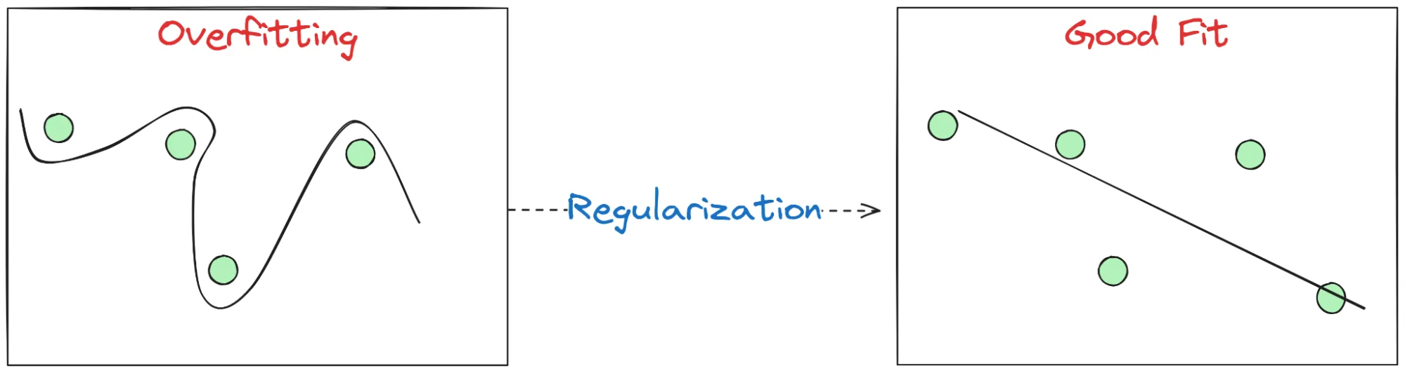
Plain English. Overfitting = great on training, poor on new data. It happens when the model uses very large, twitchy weights to chase noise.

Fix. Add a small penalty for large weights; the model still fits the data, but prefers simpler settings unless data begs otherwise.

---

2) What L2 regularization actually is

---

We add the squared size of the weights to the loss. A common definition (nice for gradients) is with a 1/2 factor:

• \(\lambda \gt 0\) controls the strength of the pull toward zero.
• We typically do not regularize the bias/intercept term.
• For classification (e.g., logistic regression), it’s the same idea—add \(\frac{\lambda}{2}\|w\|^2\) to the data loss.

---

3) From OLS to Ridge: the step-by-step math

---

Ordinary Least Squares (OLS). With design matrix \(X\in\mathbb{R}^{n\times p}\) and targets \(\mathbf{y}\in\mathbb{R}^n\):

Ridge (OLS + L2). Add \(\frac{\lambda}{2}\|\mathbf{w}\|^2\):

Setting the gradient to zero gives the closed form:

If you define OLS without the \(1/n\), the formula becomes \((X^\top X+\lambda I)^{-1}X^\top y\). Both are common; we’ll keep the \(n\lambda\) version consistent with the \(1/(2n)\) normalization above.

---

4) Gradient update & “weight decay” (why the weights shrink)

---

Gradient descent with learning rate \(\eta\) on \(\mathcal{L}_\lambda\) gives:

Key effect. Every step multiplies \(\mathbf{w}\) by \((1-\eta\lambda)\). That’s why L2 in optimizers is often called weight decay.

---

5) Geometry: ellipse meets circle (why solutions get “rounded”)

---

OLS loss contours are ellipses in weight space; the L2 constraint \(\|\mathbf{w}\|^2\le c\) is a circle (sphere in higher-D). The optimum is where the smallest ellipse first touches the circle—tangency.

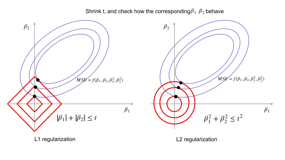
L2 vs L1. L1 is a diamond and loves corners → exact zeros (sparsity). L2 is a circle and shrinks everything smoothly (rarely exact zero).

---

6) Bayesian view: Gaussian prior ⇒ ridge

---

Assume noise \( \varepsilon\sim\mathcal{N}(0,\sigma^2I) \) and a prior \( \mathbf{w}\sim\mathcal{N}(\mathbf{0},\tau^2 I) \). Maximizing the posterior (MAP) yields ridge with \( \lambda=\sigma^2/\tau^2 \):

Interpretation. Larger noise \(\sigma^2\) or stronger belief that weights are small (small \(\tau^2\)) → bigger \(\lambda\).

---

7) SVD shrinkage: how ridge dampens weak directions

---

Let \(X=U\Sigma V^\top\) with singular values \(\sigma_1\ge\dots\ge\sigma_r\). In this basis, ridge scales components by:

Small \(\sigma_j\) (ill-conditioned directions) get shrunk most → better stability and less overfitting.

---

8) Choosing λ (practical and painless)

---

Method	How	Good starting point
Cross-validation	Scan λ on a log grid; pick best validation score	\(10^{-4}\) … \(10^{1}\)
RidgeCV	Built-in scikit-learn cross-validated ridge	Decades grid, e.g., [1e-4, …, 10]
Empirical Bayes	Maximize marginal likelihood (advanced)	Use when you know noise priors

---

9) Tiny numeric examples (feel the effect)

---

---

10) Hands-on (scikit-learn): overfit polynomial vs ridge/RidgeCV

---

import numpy as np, matplotlib.pyplot as plt
from sklearn.preprocessing import StandardScaler, PolynomialFeatures
from sklearn.linear_model import LinearRegression, Ridge, RidgeCV
from sklearn.pipeline import make_pipeline

# 1) Data: noisy sine
rng = np.random.default_rng(42)
X = np.linspace(0, 10, 80)[:, None]
y = np.sin(X).ravel() + 0.5 * rng.normal(size=80)

# 2) Overfit baseline: degree-15 OLS (no regularization)
ols = make_pipeline(StandardScaler(with_mean=False),  # keep bias out; poly adds bias if include_bias=True
                    PolynomialFeatures(15, include_bias=False),
                    LinearRegression())
ols.fit(X, y)

# 3) Ridge with a fixed alpha
ridge = make_pipeline(PolynomialFeatures(15, include_bias=False),
                      StandardScaler(),        # scale features -> crucial
                      Ridge(alpha=10.0, fit_intercept=True, random_state=0))
ridge.fit(X, y)

# 4) RidgeCV to pick alpha automatically (across decades)
alphas = np.logspace(-4, 1, 20)
ridgecv = make_pipeline(PolynomialFeatures(15, include_bias=False),
                        StandardScaler(),
                        RidgeCV(alphas=alphas, store_cv_values=False))
ridgecv.fit(X, y)
print("Best alpha from CV:", ridgecv.named_steps['ridgecv'].alpha_)

# 5) Plot
Xp = np.linspace(0, 10, 400)[:, None]
plt.figure(figsize=(8,4))
plt.scatter(X, y, s=15, c='k', label='data')
plt.plot(Xp, ols.predict(Xp),    'r--', label='deg-15 OLS (overfit)')
plt.plot(Xp, ridge.predict(Xp),  'b-',  label='deg-15 Ridge (α=10)')
plt.plot(Xp, ridgecv.predict(Xp),'g-',  label='RidgeCV (best α)')
plt.legend(); plt.tight_layout(); plt.show()

What to look for. OLS wiggles between points; Ridge yields a smoother curve; RidgeCV often lands on a value similar to what you’d choose by eye.

---

11) Hands-on (PyTorch): weight decay with proper parameter groups

---

import torch, torch.nn as nn
torch.manual_seed(0)

# Simple dataset: y = 2x + noise
N = 256
x = torch.linspace(-3, 3, N).unsqueeze(1)
y = 2*x + 0.7*torch.randn_like(x)

# Tiny model
model = nn.Sequential(nn.Linear(1, 32), nn.ReLU(), nn.Linear(32, 1))

# Parameter groups: decay weights, DON'T decay biases or norms
decay, no_decay = [], []
for name, p in model.named_parameters():
    if p.requires_grad:
        if name.endswith(".bias"):
            no_decay.append(p)
        else:
            decay.append(p)

optim = torch.optim.AdamW([
    {'params': decay,    'weight_decay': 1e-2},
    {'params': no_decay, 'weight_decay': 0.0}
], lr=1e-3)

loss_fn = nn.MSELoss()

for step in range(2000):
    optim.zero_grad()
    pred = model(x)
    loss = loss_fn(pred, y)
    loss.backward()
    optim.step()
    if step % 400 == 0:
        print(f"step {step:4d}  loss={loss.item():.4f}")

Why groups? Decaying biases/LayerNorm often hurts performance. Most training recipes decay only the “real capacity” weights (linear/conv kernels).

---

12) Common pitfalls & quick fixes

---

• Not scaling features. Fix: StandardScaler() before ridge.
• Regularizing the bias. Fix: exclude bias/intercept from L2.
• Too big λ → underfit. Training and validation both poor; reduce λ.
• Too small λ → overfit. Training great, validation poor; increase λ.
• Using Adam instead of AdamW. Prefer AdamW to decouple weight decay.

---

13) Watch: StatQuest on Ridge

---

---

14) Mini-Glossary

---

• Regularization — discourage overly complex models to improve generalization.
• L2 / Ridge — penalize squared weights; smooth shrinkage.
• L1 / Lasso — penalize absolute weights; encourages exact zeros.
• Weight decay — the optimizer form of L2: multiply weights by (1 − ηλ) each step (plus gradient).
• Bias–variance — small extra bias can reduce variance a lot → better test error.

---

15) References & Further Reading

---

1. Hoerl & Kennard (1970). Ridge Regression: Biased Estimation for Nonorthogonal Problems. Technometrics.
2. Hastie, Tibshirani, Friedman (2009). The Elements of Statistical Learning, Ch. 3 & 7.
3. Bishop (2006). Pattern Recognition and Machine Learning, Ch. 3 & 7.
4. Loshchilov & Hutter (2019). Decoupled Weight Decay Regularization (AdamW).
5. Wikipedia: Ridge regression, Tikhonov regularization, Bias–variance trade-off.

---

16) FAQ

---

Q1. Should I use L2 for classification (logistic regression)?

Yes. Add \(\frac{\lambda}{2}\|w\|^2\) to the logistic loss. It improves stability and generalization.

Q2. Do I regularize the bias?

Usually no. In scikit-learn, that’s handled automatically; in PyTorch, exclude bias/LayerNorm from weight decay via parameter groups (see code above).

Q3. Is L2 better than L1?

Different goals. L2 = stability and smooth shrinkage (keeps most features). L1 = sparsity (feature selection). Elastic Net mixes both.

Q4. How large should λ be?

Start with cross-validation over decades (\(10^{-4}\) … \(10^{1}\)), standardize features, and let RidgeCV pick the winner.