Labeled data is expensive. Unlabeled data is everywhere. Self‑supervised learning (SSL) turns the second into the first: it creates its own labels from the data itself. This guide explains SSL in plain English first, then dives into the math (entropy, cross‑entropy, KL, InfoNCE), the major families (masked modeling, contrastive, non‑contrastive), and practical systems like BERT, MAE, SimCLR, CLIP, and wav2vec 2.0. You’ll see minimal NumPy and PyTorch code, diagram placeholders, and a high‑quality video for intuition.

---

1) Self‑Supervised Learning in Plain English

---

Idea: In supervised learning, humans provide labels (cat vs. dog). In self‑supervised learning, the data provides its own supervision. We hide some part of it and train a model to predict the missing part. Over time, the model must understand structure to do well.

Analogy: Imagine covering random words in a sentence with sticky notes and asking a student to fill them in. To succeed, they must understand vocabulary, grammar, and context. That’s language modeling, the classic SSL pretext task.

---

2) Why SSL Matters

---

• Scale without labels: The web is an ocean of text, images, audio. SSL taps that ocean.
• Better features: SSL often learns robust, general features. Downstream tasks need fewer labels.
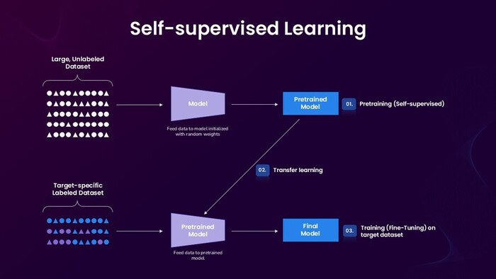
• Domain adaptation: Pretrain on large generic data; fine‑tune on your specific domain later.

---

3) Just Enough Information Theory (friendly math)

---

SSL connection: When we mask words (or image patches) and predict them, we’re reducing uncertainty (entropy) about the missing part given the visible context. We train models to minimize cross‑entropy between the true distribution and the model’s predictions.

---

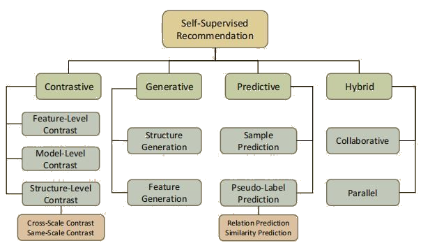
4) The Three Big Families of SSL

---

1. Predictive / Masked modeling — Hide a part, predict it (e.g., BERT masks tokens; MAE masks patches).
2. Contrastive — Pull semantically similar views together, push dissimilar apart (e.g., SimCLR, MoCo).
3. Non‑contrastive — Learn invariances without negatives, avoid collapse with architectural tricks (e.g., BYOL, SimSiam).

---

5) Masked Language Modeling (BERT‑style)

---

BERT hides ~15% of tokens and asks the model to fill them in. The loss is cross‑entropy over the masked positions:

\( \mathcal{L}_{\mathrm{MLM}} = -\sum_{t \in \mathcal{M}} \log p_\theta(x_t \mid \mathbf{x}_{\setminus \mathcal{M}})\)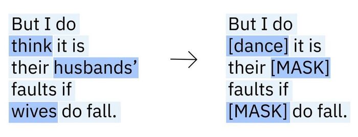

5.1 Minimal NumPy toy: mask‑and‑predict with bigrams

import numpy as np
# Tiny toy: predict a missing word from its left neighbor via bigram counts
corpus = "the cat sat on the mat the cat ate".split()
vocab = sorted(set(corpus))
ix = {w:i for i,w in enumerate(vocab)}
# Build bigram counts
C = np.zeros((len(vocab), len(vocab)), dtype=np.float32)
for a,b in zip(corpus[:-1], corpus[1:]):
    C[ix[a], ix[b]] += 1
# Turn counts into conditional probabilities p(next | prev)
row_sums = C.sum(1, keepdims=True) + 1e-8
P = C / row_sums

def predict_missing(left_word):
    if left_word not in ix: return None
    return vocab[P[ix[left_word]].argmax()]

print("Vocab:", vocab)
print("Most likely after 'the' ->", predict_missing("the"))

This is deliberately simple, but it shows the intuition: to fill in a blank, learn dependencies from context.

---

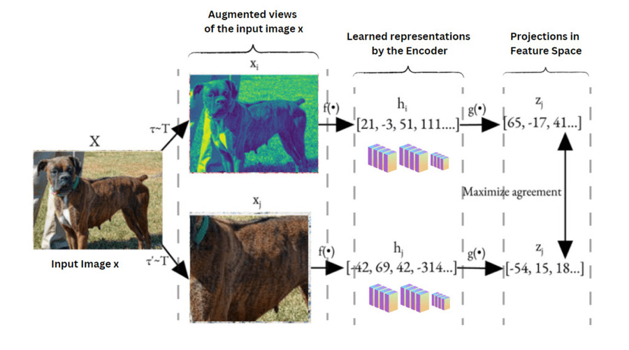
6) Contrastive Learning & InfoNCE (SimCLR, MoCo)

---

Goal: Map augmented views of the same sample to nearby vectors (positives), and of different samples to distant vectors (negatives). The InfoNCE loss for a query \(q\) and key \(k^+\) against negatives \(\{k_j\}\):

\( \mathcal{L}_{\mathrm{InfoNCE}} = -\log \frac{\exp(\mathrm{sim}(q,k^+)/\tau)} {\sum_{j} \exp(\mathrm{sim}(q,k_j)/\tau)} \)

Here \(\mathrm{sim}\) is usually cosine similarity and \(\tau\) is a temperature that controls concentration.

---

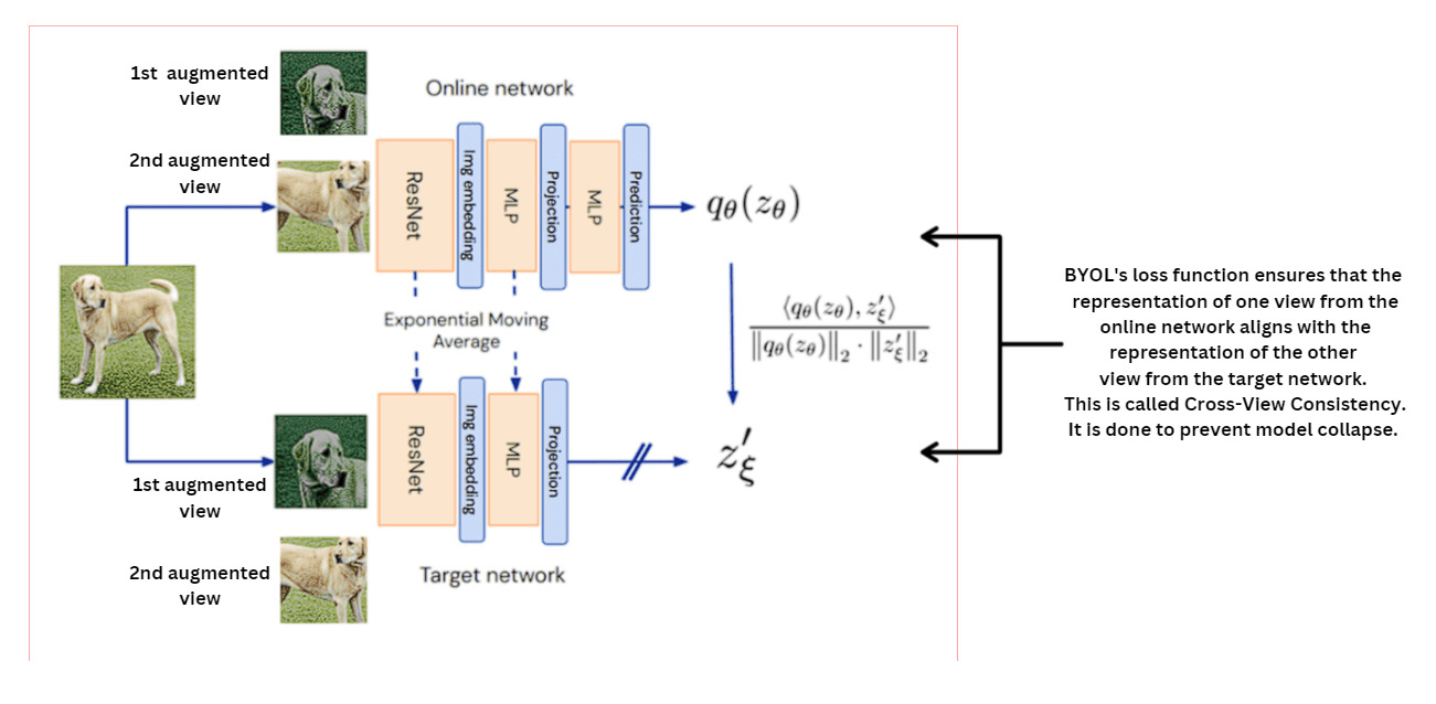
7) Non‑Contrastive SSL (BYOL, SimSiam): no negatives, no collapse

---

BYOL uses two networks: online (with a predictor) and target (an EMA copy). It brings online‑predictions close to target‑projections of another augmented view. Surprisingly, it avoids trivial collapse (constant output) without explicit negatives, thanks to architecture and the predictor/stop‑grad tricks.

---

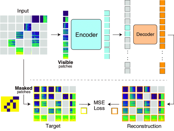
8) Vision SSL: MAE, DINO, MoCo (quick tour)

---

• MAE (Masked Autoencoders): Mask ~75% patches of an image; encode visible patches; a lightweight decoder reconstructs missing pixels. Forces strong spatial understanding.
• DINO: Self‑distillation with no labels; a student matches a teacher’s soft assignments under augmentations (vision transformers shine here).
• MoCo: Contrastive with a momentum encoder and a dictionary queue, enabling many negatives even with small batches.

---

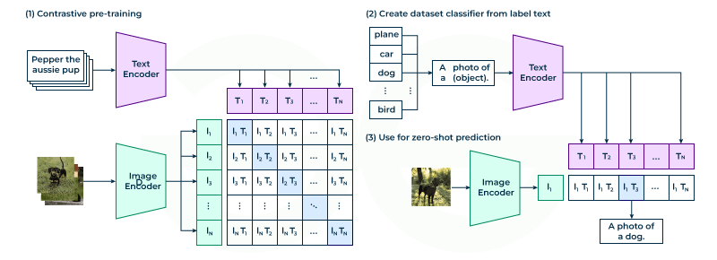
9) Multimodal & Audio SSL: CLIP, wav2vec 2.0

---

CLIP: Train an image encoder and a text encoder so that matching image–caption pairs have high similarity; non‑matching pairs are low. This aligns modalities in a shared space (zero‑shot classification emerges!).

wav2vec 2.0: SSL for speech. Mask latent audio chunks; context network predicts them; features transfer to ASR with few labels.

---

10) Hands‑On Code (minimal but meaningful)

---

10.1 Tiny HuggingFace MLM example (BERT)

# pip install transformers datasets torch
from transformers import BertTokenizerFast, BertForMaskedLM, DataCollatorForLanguageModeling
from transformers import Trainer, TrainingArguments
from datasets import load_dataset

# 1) Tokenizer & model
tok = BertTokenizerFast.from_pretrained("bert-base-uncased")
model = BertForMaskedLM.from_pretrained("bert-base-uncased")

# 2) Data: use a tiny public text dataset for demo (e.g., wikitext-2-raw-v1)
ds = load_dataset("wikitext", "wikitext-2-raw-v1")
def tok_fn(ex):
    return tok(ex["text"], truncation=True, padding="max_length", max_length=128)
tok_ds = ds.map(tok_fn, batched=True, remove_columns=ds["train"].column_names)

# 3) Data collator will randomly mask tokens as BERT's pretext task
collator = DataCollatorForLanguageModeling(tokenizer=tok, mlm_probability=0.15)

# 4) Trainer
args = TrainingArguments(
    output_dir="./mlm-demo",
    per_device_train_batch_size=16,
    per_device_eval_batch_size=16,
    eval_strategy="steps",
    logging_steps=200,
    save_steps=200,
    max_steps=1000 # small demo
)
trainer = Trainer(model=model, args=args,
                  data_collator=collator,
                  train_dataset=tok_ds["train"].select(range(5000)), # small subset
                  eval_dataset=tok_ds["validation"].select(range(1000)))
trainer.train()

10.2 Minimal SimCLR training step (sketch)

import torch, torch.nn as nn, torch.nn.functional as F

class Projection(nn.Module):
    def __init__(self, dim, proj=128):
        super().__init__()
        self.net = nn.Sequential(
            nn.Linear(dim, dim), nn.ReLU(inplace=True),
            nn.Linear(dim, proj))
    def forward(self, x): return self.net(x)

def nt_xent(z1, z2, tau=0.2):
    # z1, z2: [B, D] normalized
    B = z1.size(0)
    z = torch.cat([z1, z2], dim=0)                      # [2B, D]
    sim = torch.matmul(z, z.t()) / tau                  # [2B, 2B]
    mask = torch.eye(2*B, dtype=torch.bool, device=z.device)
    sim.masked_fill_(mask, -9e15)                       # remove self-similarity
    # positives: (i, i+B) and (i+B, i)
    pos = torch.cat([torch.arange(B, 2*B), torch.arange(0, B)]).to(z.device)
    labels = pos
    loss = F.cross_entropy(sim, labels)
    return loss

# encoder = YourBackbone()
# proj = Projection(dim=encoder_out)
# for (x1, x2) in loader:  # two augmented views per image
#   h1, h2 = encoder(x1), encoder(x2)
#   z1, z2 = F.normalize(proj(h1), dim=1), F.normalize(proj(h2), dim=1)
#   loss = nt_xent(z1, z2)

---

11) Practical Engineering Tips

---

• Augmentations are everything (vision): Color jitter, crop/resize, blur—tune carefully. Too weak → trivial; too strong → impossible.
• Temperature \(\tau\) (contrastive): Controls softness. Typical range 0.05–0.5; lower = sharper distributions.
• Batch size & negatives: SimCLR likes big batches; MoCo uses a queue. Monitor memory.
• Projection head: A small MLP often improves SSL; discard it for downstream tasks.
• Normalization: L2‑normalize features before similarity; BatchNorm/LayerNorm choices matter.
• Collapse detection: Track feature variance per dimension; near‑zero variance across a batch can signal collapse.
• Compute: SSL can be heavy; consider smaller backbones or patch‑based masking (MAE is efficient).

---

12) Ethics & Data Considerations

---

Because SSL scales on unlabeled data, curation is crucial: bias, privacy, license compliance, and content filtering all matter. Representations inherit the statistics of what they see.

---

13) A Short, Clear Video

---

---

14) Mini‑Glossary

---

• Self‑supervised learning (SSL) — Learn from the data itself via a pretext task (no human labels).
• Pretext task — An artificial task (masking, contrastive) whose solution requires learning structure.
• Contrastive learning — Bring positives together, push negatives apart (InfoNCE loss).
• Non‑contrastive — Learn invariances without explicit negatives (BYOL, SimSiam).
• Projection head — An MLP added during SSL (often removed for downstream evaluation).
• Linear probe — Train a linear classifier on frozen features to measure representation quality.

---

15) References & Further Reading

---

1. Devlin et al. (2019). BERT: Pre-training of Deep Bidirectional Transformers for Language Understanding.
2. He et al. (2020). Momentum Contrast for Unsupervised Visual Representation Learning (MoCo).
3. Chen et al. (2020). A Simple Framework for Contrastive Learning of Visual Representations (SimCLR).
4. Grill et al. (2020). Bootstrap Your Own Latent (BYOL).
5. Chen & He (2021). Exploring Simple Siamese Representation Learning (SimSiam).
6. He et al. (2022). Masked Autoencoders Are Scalable Vision Learners (MAE).
7. Radford et al. (2021). Learning Transferable Visual Models From Natural Language Supervision (CLIP).
8. Baevski et al. (2020). wav2vec 2.0: A Framework for Self-Supervised Learning of Speech Representations.
9. Mikolov et al. (2013). Efficient Estimation of Word Representations in Vector Space (word2vec).
10. Wikipedia intros for quick refreshers: Semi/SSL, Contrastive learning, Language model.