Inside the Confusion Matrix: Metrics Every Data Scientist Should Know
Nearly every classification problem ends with a confusion matrix. It looks simple—TP, FP, TN, FN—but it hides a whole ecosystem of metrics. This guide explains each one slowly and clearly: accuracy, precision, recall (sensitivity/specificity), F1 and \(F_\beta\), ROC-AUC vs PR-AUC, MCC, Cohen’s \(\kappa\), calibration & Brier score, threshold tuning, averaging (micro/macro/weighted), multi-class, and what to pick for imbalanced data. You’ll also get hands-on Python code you can run and adapt.
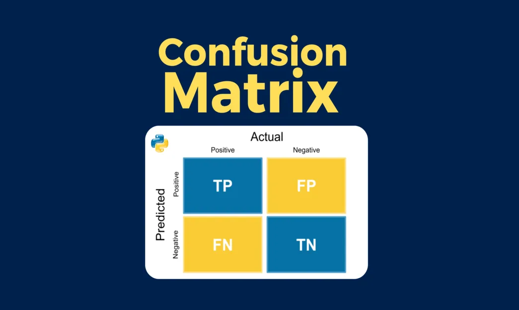
1) The Confusion Matrix
For binary classification (positive vs negative), we count:
2) Basic Rates & Formulas
From TP, FP, TN, FN we define:
3) F1 and \(F_\beta\): balancing precision & recall
F1 is the harmonic mean of precision and recall—high only when both are high.
Generalizing, \(F_\beta\) emphasizes recall (if \(\beta>1\)) or precision (if \(\beta<1\)):< /p>
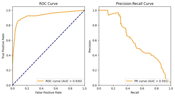
4) ROC vs PR Curves (and AUC)
Most classifiers output a probability/score. You choose a threshold \(t\) (e.g., \(0.5\)) to convert score → class. As \(t\) moves from 1→0, metrics change:
- ROC curve: plot TPR (Recall) vs FPR. ROC AUC is the area under this curve.
- PR curve: plot Precision vs Recall. Average Precision (PR AUC) summarizes the curve.
5) Matthews Correlation (MCC) & Cohen’s \(\kappa\)
MCC is a single score that stays meaningful under class imbalance (−1…+1; 0 = random; 1 = perfect):
Cohen’s \(\kappa\) compares accuracy to what you’d expect by chance agreement:
6) Calibration & Brier Score
Two classifiers can have the same ROC-AUC, but one could be better calibrated (its probabilities reflect real-world frequencies). The Brier score measures this:
Lower is better. You can visualize calibration with a reliability curve (predicted probs binned vs actual positive rate). Techniques like Platt scaling or isotonic regression improve calibration.
7) Threshold Tuning (align metrics with business costs)
Default \(t=0.5\) is arbitrary. Pick the threshold that optimizes what you care about:
- Maximize F1 if you value both precision & recall.
- Maximize precision @ target recall (or vice versa).
- Minimize cost \(C = c_{FP}\cdot FP + c_{FN}\cdot FN\) if errors have different prices.
8) Imbalanced Data & Averaging Strategies
Binary: prefer PR-AUC, MCC, recall at fixed precision, or precision at fixed recall. Consider class-weighted losses or re-sampling.
Multi-class: metrics can be averaged across classes:
- Micro: compute global TP/FP/FN and then the metric. Favors large classes.
- Macro: average metric per class equally. Treats all classes equally.
- Weighted: macro but weighted by class support. Compromise between micro and macro.
9) Multi-Class Confusion Matrix
For \(K\) classes, the confusion matrix is \(K\times K\). Row \(i\) (actual) vs column \(j\) (predicted). Diagonal = correct. Off-diagonal = confusions.
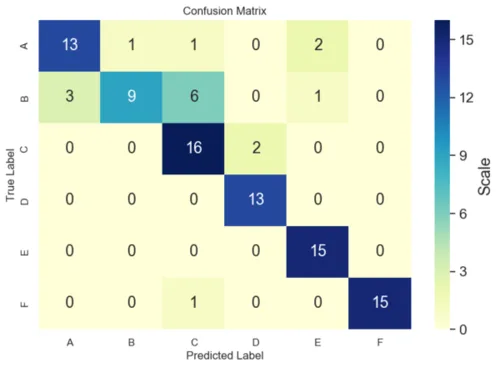
Compute per-class precision/recall/F1 by treating each class as “positive” vs “rest” (one-vs-rest), then average (micro/macro/weighted).
10) Python: End-to-End Example (binary + imbalanced)
import numpy as np
import matplotlib.pyplot as plt
from sklearn.datasets import make_classification
from sklearn.linear_model import LogisticRegression
from sklearn.metrics import (confusion_matrix, accuracy_score, precision_score, recall_score, f1_score,
                             roc_auc_score, average_precision_score, matthews_corrcoef,
                             classification_report, cohen_kappa_score, brier_score_loss,
                             precision_recall_curve, roc_curve)
from sklearn.calibration import calibration_curve
from sklearn.model_selection import train_test_split
from sklearn.preprocessing import StandardScaler

# 1) Imbalanced toy data: 5% positives
X, y = make_classification(n_samples=6000, n_features=10, n_informative=6,
                           weights=[0.95, 0.05], random_state=42)
X_train, X_test, y_train, y_test = train_test_split(X, y, test_size=0.3,
                                                    stratify=y, random_state=42)

# 2) Scale + logistic regression with class_weight='balanced' (helps imbalance)
scaler = StandardScaler().fit(X_train)
X_train_s, X_test_s = scaler.transform(X_train), scaler.transform(X_test)
clf = LogisticRegression(max_iter=200, class_weight='balanced', random_state=42)
clf.fit(X_train_s, y_train)

# 3) Scores & default threshold 0.5
proba = clf.predict_proba(X_test_s)[:, 1]
pred05 = (proba >= 0.5).astype(int)

cm = confusion_matrix(y_test, pred05)
acc = accuracy_score(y_test, pred05)
prec = precision_score(y_test, pred05)
rec = recall_score(y_test, pred05)
f1 = f1_score(y_test, pred05)
mcc = matthews_corrcoef(y_test, pred05)
kappa = cohen_kappa_score(y_test, pred05)
roc_auc = roc_auc_score(y_test, proba)
ap = average_precision_score(y_test, proba)   # PR AUC
brier = brier_score_loss(y_test, proba)

print("Confusion matrix (t=0.5):\n", cm)
print(f"Accuracy={acc:.3f}  Precision={prec:.3f}  Recall={rec:.3f}  F1={f1:.3f}")
print(f"MCC={mcc:.3f}  Kappa={kappa:.3f}  ROC-AUC={roc_auc:.3f}  PR-AUC={ap:.3f}  Brier={brier:.3f}")

print("\nPer-class report:")
print(classification_report(y_test, pred05, digits=3))

# 4) Threshold tuning via PR curve: pick threshold for target recall, e.g., 0.80
precisions, recalls, thrs = precision_recall_curve(y_test, proba)
target_recall = 0.80
idx = np.argmin(np.abs(recalls - target_recall))
t_star = thrs[max(idx-1,0)]  # thrs has length len(recalls)-1
pred_t = (proba >= t_star).astype(int)
print(f"\nChosen threshold for recall≈{target_recall}: t*={t_star:.3f}")

# 5) ROC/PR curves
fpr, tpr, _ = roc_curve(y_test, proba)
plt.figure(figsize=(11,4))
plt.subplot(1,2,1); plt.plot(fpr, tpr, label=f'ROC AUC={roc_auc:.3f}')
plt.plot([0,1],[0,1],'k--',alpha=.5); plt.xlabel('FPR'); plt.ylabel('TPR (Recall)')
plt.title('ROC Curve'); plt.legend()

plt.subplot(1,2,2); plt.plot(recalls, precisions, label=f'PR AUC={ap:.3f}')
plt.xlabel('Recall'); plt.ylabel('Precision'); plt.title('PR Curve'); plt.legend()
plt.tight_layout(); plt.show()

# 6) Calibration curve (reliability diagram)
prob_true, prob_pred = calibration_curve(y_test, proba, n_bins=10)
plt.figure(figsize=(5,4))
plt.plot(prob_pred, prob_true, 'o-', label='Model')
plt.plot([0,1],[0,1],'k--',alpha=.5, label='Perfectly calibrated')
plt.xlabel('Predicted probability'); plt.ylabel('True frequency'); plt.title('Calibration Curve')
plt.legend(); plt.tight_layout(); plt.show()
What you’ll see: On imbalanced data, accuracy can look fine while recall is poor. PR-AUC, MCC, and threshold tuning tell a fuller story. Calibration shows if your probabilities can be trusted.
11) Quick Cheatsheet (what to use when)
| Scenario | Prefer | Why |
|---|---|---|
| Balanced binary task | Accuracy, ROC-AUC, F1 | All classes represented; ROC-AUC summarizes ranking. |
| Imbalanced (rare positives) | PR-AUC, Recall@Precision, MCC, F1/F\(_\beta\) | Focus on retrieving positives with controlled false alarms. |
| Business costs differ (FN ≫ FP or vice versa) | Cost-weighted objective, threshold tuning | Pick \(t\) that minimizes expected cost. |
| Multi-class; minority classes matter | Macro F1, per-class metrics, confusion heatmap | Treats all classes equally; makes confusions visible. |
| Need trustworthy probabilities | Calibration curve, Brier score | Good for decision thresholds and risk scoring. |
12) Mini-Glossary (jargon → plain English)
- Confusion matrix — 2×2 table of TP, FP, TN, FN.
- Precision (PPV) — of predicted positives, how many were correct?
- Recall (Sensitivity, TPR) — of actual positives, how many did we find?
- Specificity (TNR) — of actual negatives, how many did we keep as negative?
- F1/F\(_\beta\) — harmonic mean(s) balancing precision & recall.
- ROC-AUC — probability a random positive ranks above a random negative.
- PR-AUC (Average Precision) — area under precision-recall curve.
- MCC — correlation-like summary robust to imbalance.
- Cohen’s \(\kappa\) — accuracy vs chance-level agreement.
- Calibration — do probabilities match real frequencies?
13) References & Further Reading
- Wikipedia: Confusion matrix, Precision and recall, ROC curve, AUC, Sensitivity & Specificity, Matthews correlation coefficient, Cohen’s kappa, Brier score.
- Hastie, Tibshirani, Friedman. The Elements of Statistical Learning — Ch. 2 (classification basics), Ch. 7 (model assessment).
- Bishop, C.M. Pattern Recognition and Machine Learning — Ch. 4–8 (classification & evaluation).
- Saito & Rehmsmeier (2015). “The Precision-Recall Plot Is More Informative than the ROC Plot When Evaluating Binary Classifiers on Imbalanced Datasets.”
14) FAQ
Q1. Why is my accuracy high but F1 low?
Imbalance. Your model predicts the majority class well but misses many positives. Look at recall, precision, PR-AUC, MCC, and tune the threshold.
Q2. ROC-AUC vs PR-AUC—which should I report?
Balanced classes → ROC-AUC is fine. Rare positives → PR-AUC better reflects usefulness because it tracks precision at various recalls.
Q3. How do I choose a threshold?
Use validation curves: maximize F1 or pick the smallest threshold that achieves a target recall/precision, or minimize cost with class-specific penalties.
Q4. What about multi-label problems?
Compute metrics per label (treat each as binary) then micro/macro/weighted average. Also consider ranking metrics (mAP) if you predict top-k labels.
Q5. My probabilities aren’t trustworthy—fix?
Try calibration: Platt scaling (logistic) or isotonic regression on a validation set; re-check the calibration curve and Brier score.
Comments